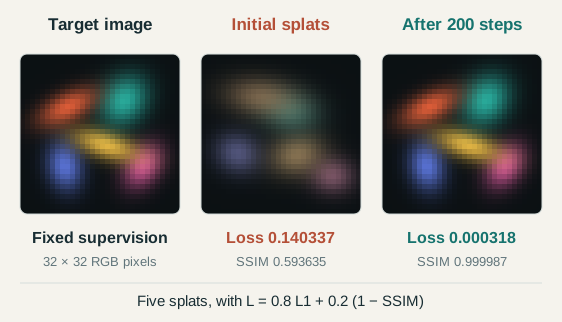
The original 2023 method learns an explicit radiance field from calibrated photographs. No photograph contains a ground-truth list of Gaussian centers or covariances. Training renders a candidate scene, measures image error and differentiates that error through the renderer. The first laboratory optimizes a small 2D Gaussian scene using the same photometric objective. The second laboratory isolates 3D position observability with orthographic cameras. Both calculate their updates from image residuals. They are teaching models, not reproductions of the CUDA pipeline. The preview uses actual optimization results from the first laboratory.
The lesson follows the causal order of the calculation: parameters determine a rendered image, the image determines a scalar loss, and the loss supplies derivatives for the parameter update. The final section asks what information the observations can identify. Read Notes expands every slide with assumptions and primary references. The two live laboratories can also be opened as responsive pages on a smaller screen.
Every camera renders the same trainable Gaussians.
The original reconstruction fixes the cameras and optimizes the scene.
Explanation and assumptions
SfM, often through COLMAP, supplies a sparse point cloud and calibrated image poses in one coordinate system. These points seed the means and colors of the initial Gaussians. The original 3DGS task treats the camera calibration as input. This deck does not describe jointly solving poses as in SLAM. Across iterations, a sampled camera changes which photograph supervises the shared Gaussian scene. There is no target splat list and no required point-to-point correspondence between a learned Gaussian and a true surface point.
The stored scales are log-scales and the stored opacity is a logit. Exponentiation produces strictly positive axis lengths and a sigmoid produces opacity between zero and one. A normalized nonzero quaternion supplies a rotation. These choices keep the covariance positive definite while allowing anisotropy. The color is represented by spherical harmonics in the original method, rather than a single fixed RGB triplet. The 2D teaching laboratory keeps constant RGB, uses a 2D angle instead of a 3D quaternion, and optimizes sigmoid RGB values. Those appearance constraints are simplifications of the original renderer.
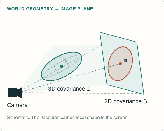
J is the 2 × 3 Jacobian of perspective projection.
Explanation and assumptions
The projection Jacobian is J=[fx/Z,0,−fx X/Z²; 0,fy/Z,−fy Y/Z²]. The covariance equation is a first-order local affine approximation. Perspective projection does not globally preserve a Gaussian density. The reference rasterizer additionally adds a 0.3 pixel-squared diagonal filter to the screen covariance. Both the projected mean and projected covariance depend on the 3D position. A full position derivative therefore includes more than the projected-mean path. The 2D lab begins directly with screen-space ellipses and does not implement this perspective stage.
The learned opacity \(o_i\) belongs to the Gaussian.
The alpha \(\alpha_i(p)\) varies across pixels.
No \(1/\sqrt{\det S_i}\) density-normalization factor appears.
Widening a splat changes how many pixels it influences.
Explanation and assumptions
The Gaussian here is an unnormalized rendering kernel. Treating it as a normalized probability density would change how scale affects brightness and would produce different gradients. In the reference implementation, alpha is capped at 0.99, negligible contributions below 1/255 are skipped and almost-opaque pixels terminate traversal. These implementation thresholds create boundaries in the otherwise smooth calculation. The teaching lab evaluates the full smooth footprints at a fixed order without the production culling and early-termination thresholds.
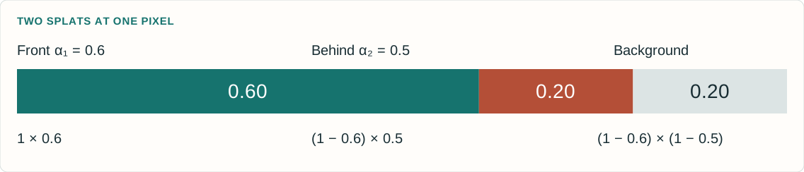
Here b is the background color and the splats are ordered from front to back for the pixel. For two splats with alpha values 0.6 and 0.5, the first contributes 0.6 of its color. The second receives transmittance 0.4 and therefore contributes 0.2. The remaining background weight is 0.2. The weights sum to one when the background term is included. Raising a front opacity changes both its own contribution and the visibility of all the color behind it. Original 3DGS uses tile binning and sorting for an efficient approximate visibility order.
An iteration samples a camera and differentiates its image loss.
WHAT THE LOSS SEES
The rendered pixels and observed pixels.
It never receives the correct Gaussian center, shape or count.
Explanation and assumptions
The reference code computes (1−lambda_dssim) times L1 plus lambda_dssim times (1−SSIM), with lambda_dssim=0.2 by default. Its D-SSIM convention has no extra factor of one-half. Other texts sometimes define DSSIM as (1−SSIM)/2, so the convention needs to be stated. The full objective can be understood as an average over training views, while the implementation samples individual cameras. Optional depth regularization and exposure-related features in later repository revisions are not part of the original 2023 base loss explained here.
At exactly zero residual, a zero subgradient is a common choice.
Explanation and assumptions
L1 loss measures the mean absolute difference across every pixel and RGB channel. A corresponding image gradient has a sign determined by whether the prediction exceeds or falls below the observation. The factor 1/(3HW) normalizes image size. This derivative is the starting signal for backpropagation, not yet a direction in world space. The renderer decides which parameter changes could create the desired pixel change. A change that helps one pixel can hurt others, and their contributions combine in the parameter gradient.
11 × 11 Gaussian window, standard deviation 1.5 pixels.
\(C_1=0.01^2,\quad C_2=0.03^2\) for images scaled to [0,1].
Average the SSIM map over windows and channels.
Explanation and assumptions
For a window, x contains predicted pixel values and y the corresponding target values. The normalized Gaussian weights define local averages and second moments. The numerator rewards agreement in means and covariance while the denominator normalizes brightness and contrast. Positive constants stabilize nearly constant or dark windows. The official unfused implementation uses zero padding for convolution, with an 11×11 window of standard deviation 1.5. Its gradient couples neighboring pixels through these statistics. The teaching laboratory implements the same local-window construction and explicitly differentiates its operations. SSIM is a structural image similarity objective, not an independent depth or surface constraint.
An illustrative calculation makes the scalar loss explicit.
MEAN ABSOLUTE RGB ERROR
0.10
Weight: 0.8
SSIM = 0.75
0.25
1 − SSIM, weight: 0.2
COMBINED LOSS
0.13
0.8 × 0.10 + 0.2 × 0.25
A COEFFICIENT IS NOT A FRACTION OF LEARNING
The relative effect also depends on each term’s magnitude and derivative.
Changing λ changes both the scalar loss and the direction of the parameter update.
Explanation and assumptions
These are illustrative input values, not a benchmark measurement. If L1=0.10 and SSIM=0.75, then the reference default gives 0.8×0.10+0.2×(1−0.75)=0.13. The coefficient 0.8 does not mean exactly 80 percent of the optimization comes from L1, because the terms have different derivatives and scales. The first lab recomputes all components from its actual images and permits changing lambda. Loss values measured under different lambda settings are different objectives and should not be read as a single continuous convergence curve.
r is the RGB loss gradient. \(C_{>i}\) is the composited color behind this splat, including the background.
Explanation and assumptions
Hold the current depth order fixed and write the pixel as C_before+T_i[alpha_i c_i+(1−alpha_i)C_tail]. Differentiating gives dI/dalpha_i=T_i(c_i−C_tail) and dI/dc_i=T_i alpha_i times the RGB identity. Thus increasing alpha replaces some tail color with the splat color. Whether this helps depends on the loss gradient and their color difference, not just on whether the pixel is dark. The transmittance factor attenuates gradients to occluded splats. This slide is an independent derivation of the compositing equation. The CUDA backward kernel implements the corresponding derivative with its own numerical and visibility bookkeeping.
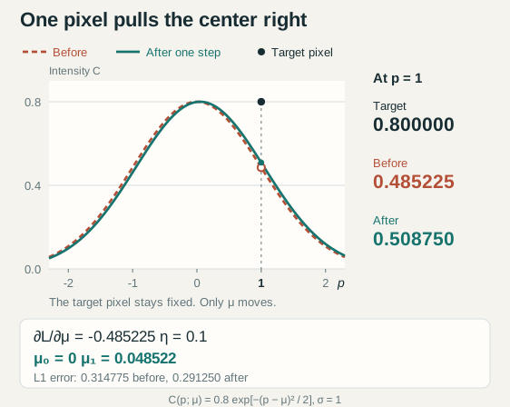
The single pixel is at p=1, the center is initially m=0, standard deviation is one, opacity is 0.8, color is one and the background is black. The target is 0.8. For this one residual, dL/dI=−1 and dI/dm=I(p−m)/s²=0.4852245, hence the center derivative is negative. Gradient descent with step size 0.1 increases the center to 0.04852245, raises the predicted pixel to 0.5087501167 and reduces absolute error to 0.2912498833. The step follows an image-loss derivative. It does not use a target center. This tiny example cannot identify every splat parameter and does not imply that every Adam step in the full nonconvex problem decreases loss.
Sum the chain-rule contributions across the image and sampled views.
WHY SPLATS DO NOT JUST GROW
A larger footprint can brighten a missed foreground pixel.
It can also spill color into a background pixel that was already correct.
The competing gradients shape the ellipse and its opacity.
Explanation and assumptions
The center derivative shown here holds the screen covariance fixed. The full 3D center derivative also includes the projected covariance and view-dependent appearance paths. For an unnormalized footprint, the screen-covariance derivative is alpha/2 times S inverse d d transpose S inverse. A positive opacity change affects every pixel under the footprint, and a scale change redistributes coverage. The desired update is the aggregate of those image effects. Soft overlapping footprints make small changes visible to the objective, but a Gaussian far from all residual support can still receive weak gradients.
The next camera then evaluates those changed parameters from another viewpoint.
1 · SAMPLE A CAMERA
Choose its observed image and fixed calibration.
2 · RENDER
Project, sort and alpha-composite the current scene.
3 · MEASURE THE LOSS
Average RGB error and local structural dissimilarity.
4 · BACKPROPAGATE
Differentiate through the evaluated rendering operations.
5 · UPDATE WITH ADAM
Change the continuous Gaussian parameters.
6 · ADAPT CAPACITY
Periodically clone, split or prune Gaussians.
Explanation and assumptions
This is a conceptual ordering of the learning loop. The exact code interleaves bookkeeping, densification and optimizer updates, so a density-control iteration need not follow this schematic order literally. Adam uses running estimates of gradient moments and group-specific learning rates. The basic descent form theta_new=theta−eta grad L explains direction, but it is not the full Adam update. Discrete density changes alter the number of variables and are handled separately from ordinary differentiation. Visibility sorting, culling and thresholds mean the full renderer is not globally smooth across every possible scene change.
Every point on the loss curve comes from a fresh render and a real update.
TRY THIS
Press Train 50, then repeat.
Compare the current render with the target and fixed-scale absolute residual.
Reset and freeze position or shape to see what the remaining variables can compensate for.
MODEL BOUNDARY
2D anisotropic Gaussians, constant RGB and a fixed front-to-back order.
Mean L1 plus local 11 × 11 SSIM, with analytic gradients and Adam.
No perspective projection, spherical harmonics or adaptive densification.
Explanation and assumptions
The lab isolates the parameter-to-image-to-loss-to-update mechanism. Its target is generated once from a hidden synthetic scene. Optimization receives the target image, not the generating parameters. A perturbed initialization is used so useful gradients reach the footprints. The data are noiseless and the model has enough capacity, which makes convergence easy to inspect. The teaching optimizer uses explicit stability bounds and decaying, group-specific learning rates. These favorable conditions are deliberate and do not establish real-world accuracy or guarantee convergence from arbitrary random initialization. Changing lambda or the active parameter groups starts a new optimization phase in the displayed history. Footprint outlines show geometry for inspection and are not part of the loss.
This live 2D teaching model computes its own render, exact loss components and analytic gradients. It does not replay a prerecorded curve or interpolate hidden target parameters. Start with all parameter groups active and lambda=0.2, then change one condition at a time after Reset. All displayed error images use a fixed scale. The full-size lab includes the model assumptions and keyboard-accessible controls.
A better image need not recover the generating parameters
Several parameters can explain some of the same pixel changes.
WHAT THE LAB ESTABLISHES
The loss is computed from the image.
Its gradient can improve the rendered prediction.
Freezing parameters changes which errors the model can correct.
WHAT IT CANNOT ESTABLISH
A unique true set of centers, colors or opacities.
For one splat on black, color and opacity can trade off through their product.
Real-world 3D reconstruction quality from a tiny 2D image fit.
Explanation and assumptions
For a single constant-color splat on a black background, the rendered image is the product of its color, opacity and footprint. Different color-opacity pairs can give the same product within valid ranges. Overlap and background change that ambiguity but do not make every parameterization uniquely identifiable. It is therefore more meaningful to inspect predicted images and held-out views than to demand that every learned primitive match a hidden synthetic parameter list. The lab can display residual and component losses without claiming exact scene recovery.
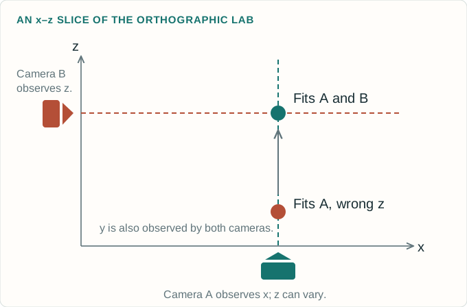
A second view checks where the splat really projects
The same 3D center must satisfy both camera images.
SHARED 3D PARAMETERS
One projection can agree while depth remains wrong.
Another camera converts that depth error into a visible image displacement.
Useful parallax makes some previously invisible parameter changes observable.
Explanation and assumptions
For a perspective camera, a center can move along a viewing ray while keeping its projected mean fixed, and a corresponding covariance change can preserve its footprint. A second noncoincident camera generally changes that projection. The next lab uses a simpler exact construction: camera A observes (x,y), camera B observes (z,y), and a held-out oblique camera observes a combination of x and z. With only A, z never enters the rendering equation. No optimizer can infer it from that image. With A and B, all three center coordinates affect the observations under the lab’s known-shape assumptions. This isolates observability rather than solving arbitrary scene geometry.
The second camera changes which center coordinates the loss can constrain.
THE EXPERIMENT
Train with one view. Watch its error fall while the unobserved depth stays wrong.
Add two views and continue from that same center.
Compare the held-out oblique image before and after.
CONTROLLED ASSUMPTIONS
One 3D isotropic Gaussian.
Known opacity, color and covariance.
Known orthographic cameras.
Only the three center coordinates are learned.
Explanation and assumptions
The target images are synthetic observations generated once. The optimizer compares only the selected training images. The held-out view and optional reference-center visualization are used for evaluation, never for training. In a fresh one-camera run, the depth derivative is exactly zero and z remains at its initial value. Switching back to one camera later freezes the current z. With the second camera enabled, z acquires a gradient. Keeping shape and appearance fixed prevents other ambiguities from obscuring this one. Real scenes involve occlusion, uncertain camera poses, anisotropic covariance and view-dependent color, so two views do not guarantee unique full-scene recovery.
This lab optimizes only the center of a known isotropic Gaussian from synthetic RGB target images, using calibrated orthographic projections. It uses the same combined photometric loss as the first lab. The single-view z gradient is zero by construction. Adding the second view permits image-loss optimization of z and improves a separate oblique view in the standard scenario. The reference center is evaluation information only. This is a local identifiability example, not a proof that all Gaussian scenes are identifiable.
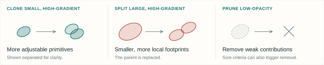
Original 3DGS periodically changes the number of primitives.
WHERE TO ADD CAPACITY
Large average screen-position gradient magnitudes flag regions the current representation struggles to fit.
A SEPARATE HEURISTIC
Clone, split and prune change the model. They are discrete operations, not another term in the image loss.
Explanation and assumptions
The reference method accumulates screen-space center gradient magnitudes and divides by the number of visible observations. High-average-gradient small Gaussians are cloned, while high-average-gradient large Gaussians are split. Very low opacity and certain excessive-size conditions cause pruning. The paper describes moving clones along a gradient direction, while the released densify_and_clone copies positions directly and lets subsequent optimization separate them. Split children are sampled around a parent and receive smaller scales. Typical reference defaults activate densification after iteration 500, repeat every 100 and stop at 15000, with opacity reset every 3000. Reset clamps opacity down to at most 0.01. These are implementation settings, not universal constants, and the browser labs do not implement density control.
Textureless areas, reflections or changing lighting.
Nonconvex optimization and redundant splat configurations.
Explanation and assumptions
The original paper reports artifacts in poorly observed regions, elongated or splotchy Gaussians and visibility-order popping. The image objective constrains rendered appearance under the available observations. Unseen regions remain weakly constrained, and different representations can explain the same finite set of photos. View-dependent color improves appearance modeling but also increases flexibility. Optimization is nonconvex, and discrete sorting and density operations introduce further complexity. “Correct splats” therefore means a representation that explains the observed images and behaves well from new views under the chosen assumptions, rather than guaranteed recovery of a unique physical decomposition.
Images supply the error. Rendering supplies the direction.
A practical explanation of why the learned splats can become useful.
HOW THE LOSS IS CONSTRUCTED
Render the calibrated camera, compare each RGB pixel, compare local image structure, then form \(0.8\mathcal L_1+0.2(1-\mathrm{SSIM})\).
HOW THAT CHANGES THE SPLATS
Backpropagate through compositing, Gaussian footprints and projection. Adam updates the parameters that produced the image error.
HOW TO JUDGE THE RESULT
Use different cameras to constrain one scene, add or remove splats as needed, and inspect held-out views. Image agreement is a test, not a uniqueness guarantee.
Explanation and assumptions
A useful diagnostic follows the computational graph. First verify the photograph-to-camera alignment and pixel range. Then inspect the rendered image, residual map and separate L1/SSIM terms. Confirm that useful gradients reach visible primitives and that parameter activations are valid. Compare active groups to understand compensation. Finally evaluate cameras that were not used in training and look for unobserved or weakly constrained regions. A falling scalar loss is helpful, but its meaning depends on a correct renderer, camera model, supervision and sufficient coverage. The labs make these mechanisms inspectable at a small scale.
The original paper is 3D Gaussian Splatting for Real-Time Radiance Field Rendering by Bernhard Kerbl, Georgios Kopanas, Thomas Leimkühler and George Drettakis, ACM Transactions on Graphics / SIGGRAPH 2023. The official repositories are the primary references for the exact loss convention and implementation details. The current code contains later optional features, so this lesson separates those from the original method. The derivations, diagrams and browser numerical models are educational work created for this site. They do not reproduce a benchmark or ship the authors’ CUDA software.