One multipath measurement, two geometries: the virtual anchor and the incidence point
A reflected radio path hands you four numbers: a delay (a path length), an arrival angle at the UE, a departure angle at the BS, and a pathloss. Read the delay and angle one way — walk the full measured length along the arrival direction — and you get a virtual anchor: a fictitious, wall-agnostic transmitter that BP-SLAM treats as a static feature. Read them the other way — stop where the arrival ray crosses the delay ellipse whose foci are the BS and the UE — and you get the incidence point: the physical spot on the wall where the ray actually bounced. Same data, two maps.
Gaussian_Splatting_Test pipeline. The virtual-anchor reading is the feature model of E. Leitinger et al., “A Belief Propagation Algorithm for Multipath-Based SLAM,” IEEE Trans. Wireless Commun. 18(12), 2019; the anchor-mirroring idea goes back to Channel-SLAM (Gentner et al., IEEE TWC 15(9), 2016). Scene and numbers here are illustrative (scale: 1 px ≙ 0.1 m).01Measurement
For one multipath component the channel estimator (SAGE, ESPRIT, …) returns a tuple (τ, φ, ψ, PL). Each element has its own geometric meaning:
angle φ (AoA at the UE)
angle ψ (AoD at the BS)
pathloss → a weight
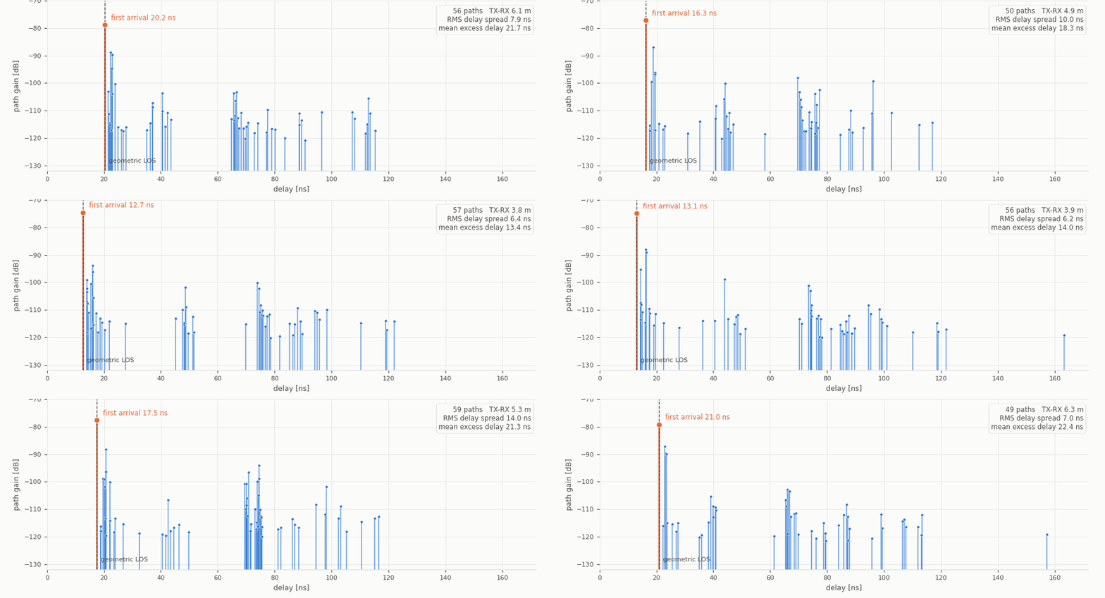
What are the factors, in addition to the distance, that affect the pathloss?
- Interaction loss at each bounce (dominant). Paths with the same travel distance span ~20 dB of excess loss. What differs is what they hit — which surface, how many times, specular vs. diffuse.
- Material and incidence angle, evidenced by polarization. On matched reflected paths, half of all matched pairs differ by more than 3 dB between polarizations.
- Small-scale / rough-surface effects.
- Blockage / shadowing. Some clusters vanish for whole stretches of frames in the delay–frame waterfall while the geometry barely changes.
02Filter view with known UE position
2.1Single bounce: draw everything from (τ, φ, ψ)
the data (drives the drawing)
layers
2.2Double bounce: two virtual anchors, two incidence points
the data — path 1 (single bounce)
the data — path 2 (double bounce)
construction — step
2.3Triple bounce: the recursion run in full
the data — path 1 (single bounce)
the data — path 2 (double bounce)
the data — path 3 (triple bounce)
construction — step
2.4Double bounce, corridor edition: two parallel walls
the data — path 1 (single bounce)
the data — path 2 (double bounce)
construction — step
2.5Triple bounce, corridor edition: parity, and a hypothesis that angles cannot kill
the data — path 1 (single bounce)
the data — path 2 (double bounce)
the data — path 3 (triple bounce)
construction — step
2.6Estimating the map: motion collapses the family
the unknown split
layers
motion, step by step
03Optimization view with unknown UE position
One quiet assumption still runs through §3.1–3.5: delays are true ranges (synchronized clocks). The other classic assumption — that array orientations are known, so ψ and φ can be drawn as global directions — is only half fair. The BS earns it: infrastructure knows which way it faces. The UE does not: its heading is one more unknown per pose, so every demo below carries a heading-hypothesis slider δ that rotates all arrival rays by a common guess. Watch what it does. In the corner scenes every construction stays perfectly coherent for every δ — the one-parameter slide becomes a two-parameter family (P⁽¹⁾, δ), and §3.1’s candidate line fattens into the whole delay disk. In the corridor scenes a wrong δ wedges the recovered walls out of parallel, yet the wedge still closes at the sliding UE₁ — heading error is indistinguishable from wall tilt. Angles measured without a compass buy geometry only relative to that compass. §3.6 draws the consequence: it never uses arrival angles to build geometry at all — wall directions come from motion, offsets from the one link that crosses the families, and each pose’s heading is read off last, from the recovered geometry.
3.1Single bounce: draw everything from (τ, φ, ψ)
the data (drives the drawing)
construction — step
3.2Double bounce: two virtual anchors, two incidence points
the data — path 1 (single bounce)
the data — path 2 (double bounce)
construction — step
3.3Triple bounce: the recursion run in full
the data — path 3 (triple bounce)
construction — step
3.4Double bounce, corridor edition: two parallel walls
the data — path 2 (double bounce)
construction — step
3.5Triple bounce, corridor edition: parity, and a hypothesis that angles cannot kill
the data — path 3 (triple bounce)
construction — step
3.6Estimating jointly: motion collapses the family — the optimization view
§2.6 collapsed the VA family by motion with known poses. Here nothing is known: not the walls, not the trajectory, not even which way the UE is facing — only each path's delay and BS-side departure angle, the UE's local arrival angles, and the relative motion between poses (odometry). This is the graphSLAM setting: every unknown enters one joint problem. Without a heading, §3.1's bisector is out of reach, and a single snapshot leaves a two-parameter family per wall — direction and offset. Motion pays that bill in two installments: odometry within a family buys the wall's direction (and throws in a parity check for free); the one link across the families buys both offsets — exactly when the walls disagree in orientation.
the unknown split — two families
layers
corridor edition — the family that survives the graph
layers
04Why the diffuse case decides the representation
With smooth walls the two readings are equivalent bookkeeping. Rough walls break the tie. A diffuse surface returns energy from a whole patch, not a point: the measurement becomes a family of slightly different (τ, φ, ψ, PL) tuples. Map those into incidence points and you get a weighted point cloud hugging the physical wall — each point carrying its pathloss as a weight. Exactly the kind of data a splat-style surface representation wants (this is what the point-cloud view in Gaussian_Splatting_Test exports, and what the SAGE bistatic triangulation estimates). Map the same family into virtual anchors and the crisp mirror-image anchor smears into a blob that no longer behaves like a point feature — the VA cloud in the demo above.
| Virtual anchor (BP-SLAM) | Incidence point (this pipeline) | |
|---|---|---|
| construction | walk the full length L along the AoA ray | stop where the AoA ray crosses the delay ellipse (foci BS & UE; for bounce n ≥ 2: foci VAⁿ⁻¹ & UE) |
| needs walls? | no — wall-agnostic, that is its superpower | no wall model either, but multi-bounce needs the previous-order VA (a hypothesis about the bounce sequence) |
| as the UE moves | fixed — behaves like a static LOS anchor, ideal as a SLAM feature with BP data association | slides along the surface — successive positions paint the wall |
| double bounce | still one clean point: VA² = mirror(mirror(BS, A), B) | two points P₁, P₂; naive BS–UE ellipse fails, VA¹–UE ellipse fixes it |
| triple bounce | still one clean point: VA³ = mirror³(BS) — the full-length walk lands on it regardless of bounce order | three points P₁, P₂, P₃; the end bounces are picked by the measured AoA/AoD, the middle bounce only by map (aim at VA²) — order n leaves n−2 map-picked bounces |
| diffuse walls | anchor smears into a cloud — point-feature model degrades | cloud lands on the wall — weighted by pathloss, it is a surface sample: a splat |
| natural output | anchor map + UE trajectory (positioning) | surface point cloud (environment mapping / Gaussian splatting) |