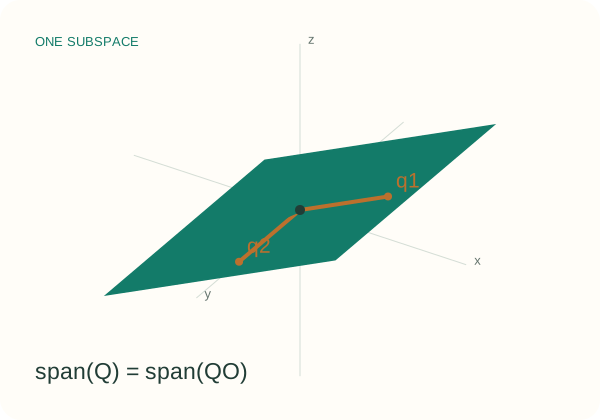
The plane is the object. A basis is its coordinate system.
We write Gr(k,n) for the set of k-dimensional linear subspaces of ℝⁿ, with 0 < k < n. All these subspaces contain the origin. Our notation puts the subspace dimension first; some references use Gr(n,k).
Many matrices, one point
Columns of Q form an orthonormal basis. Multiplying by an orthogonal O rotates or reflects that basis without changing its span. The quotient identifies all such matrices.
A unique projector
P is the orthogonal projector onto the subspace. For a vector x, Px is its least-squares projection. The trace of P equals k.
The Stiefel manifold St(k,n) keeps the particular ordered orthonormal frame Q. The Grassmannian removes its k(k−1)/2 internal rotational degrees of freedom:
Gr(1,3) is the real projective plane: a unit vector and its negative define the same line. It is not the sphere itself. Gr(2,3) can similarly be represented by a plane normal with n and −n identified. An offset plane belongs to the affine Grassmannian.
Principal angles remove the choice of basis.
Subtracting two basis matrices measures their coordinate choices as well as their geometry. Instead, compare how well their directions align.
The first angle finds the best-aligned pair of unit vectors, one from each subspace. Subsequent pairs are constrained to be orthogonal to the previously chosen directions. Singular values make the result invariant to independent basis rotations.
Intrinsic geodesic distance
Use angles in radians. This is the shortest path length for the canonical Grassmann metric, whose horizontal tangent inner product is the Frobenius inner product.
Projection distance
A distance in projector coordinates. It approximates dg for small angles but is not the same global quantity. We name the normalization explicitly because “chordal” conventions vary.
Why use Gr(2,4) here? Two planes in ℝ³ intersect in at least a line, so their first principal angle is always zero. Four dimensions allow both angles to vary independently.
A tangent changes the subspace, then a curve stays on it.
Horizontal tangent
QΩ with skew-symmetric Ω rotates the basis inside its current subspace. A horizontal Δ moves toward the orthogonal complement and represents a tangent to the quotient.
Metric convention
In projector coordinates the corresponding metric is one half of the Frobenius inner product. Keeping this factor is what makes the geodesic distance equal to ‖θ‖₂.
For a compact SVD Δ = UΣVᵀ of rank r, the exponential map has an orthonormal representative
It starts at Q with velocity Δ. Sines and cosines rotate each active direction toward the orthogonal complement. The curve remains defined beyond the shortest-path interval; the distance from the start need not then equal its traveled length.
A local logarithm
When QᵀY is invertible, form
This is a horizontal representative. At a principal angle of π/2 the inverse fails and a shortest logarithm is not unique. Near this boundary, use numerically robust algorithms from the handbook.
A practical retraction
QR orthonormalization provides a cheaper local approximation with the correct first-order behavior. It represents a subspace regardless of QR column signs. A retraction is generally not the exact exponential map.
PCA learns a subspace, not a particular basis.
For centered data with covariance C, the best rank-k orthogonal reconstruction maximizes captured variance.
The objective is unchanged under Q → QO. Project the Euclidean gradient to the horizontal tangent, take a step, then retract. Our lab uses backtracking to require sufficient improvement. The leading k-dimensional eigenspace gives an independent reference solution.
A repeated eigenvalue within the selected subspace does not destroy uniqueness of that subspace. What matters is the boundary gap λk > λk+1. The same geometric viewpoint appears in subspace tracking, reduced models, and signal processing.
For complex signal subspaces, replace Qᵀ by Qᴴ and O(k) by U(k). The complex Grassmannian has complex dimension k(n−k), or real dimension 2k(n−k). All five labs on this page use real matrices.
Global data association with lines and planes.
Lusk & How (2022), “Global Data Association for SLAM with 3D Grassmannian Manifold Objects”, builds a consistency graph from affine objects in two lidar scans. The association step needs no initial relative-pose guess.
From linear to affine
A 3-D line uses k = 1; a plane uses k = 2. Translation along the object does not create a new affine subspace. Its dimension is (k+1)(n−k).
These orthonormal coordinates embed Graff(k,3) into Gr(k+1,4). Our coordinates are made dimensionless by dividing positions by a length scale ρ.
Shift before embedding
Directly applying the embedding depends on the global origin. For a pair, the paper first shifts both stored affine anchors by −b₁:
Only then compute the perpendicular displacement and the embedding. Under a shared rigid transform, this relative displacement rotates but the translation cancels. Compare the same ordered pair in both scans.
Lab experiment: change the translation, then switch between shifted and raw affine descriptors.
- Generate candidates. A vertex represents Aᵢ ↔ Bⱼ. Only same-type matches are candidates: lines match lines and planes match planes.
- Compare pairs inside each scan. For candidates u = (i,j) and v = (p,q), compute c = |d(Aᵢ,Aₚ) − d(Bⱼ,Bq)|. These within-scan pairs may mix a line and a plane.
- Score compatibility. Keep an edge if c < ε, with weight exp(−c²/(2σ²)). Reusing either source or target object makes an edge forbidden. Set the diagonal to one.
- Select a consistent set. Maximize uᵀMu/uᵀu over nonempty binary selections with no forbidden pairs. Weighted density can favor a smaller, stronger clique over a larger, weaker one.
- Estimate the transform. The paper then aligns matched lines and planes by least squares. This final registration stage is outside this association lab.
For mixed object dimensions, the paper uses the norm of the min(k₁+1,k₂+1) principal angles. It can be zero for containment between different dimensions; it is not a separating metric on their union. Same-type candidate matching and mixed-type pairwise consistency are different operations.
What the demo implements
The affine embedding, pair shift and scale, consistency weights, one-to-one exclusions, and discrete density objective follow equations (2)–(5), (8)–(9), and Proposition 1 of the supplied paper. Every feasible clique is enumerated on this small graph, including nonmaximal cliques. The paper uses the scalable CLIPPER relaxation. This browser experiment uses synthetic objects and transformed anchors, without lidar segmentation, pose estimation, or a KITTI benchmark. Ground-truth identities are used only for reporting recovery, never for scoring or selection.
Our scene uses ρ = 3 m, ε = 0.16 rad and σ = 0.05 rad. The paper reports ρ = 40 m, ε = 0.2 and σ = 0.02 for its KITTI experiments. Anchor perturbations and direction noise are explicit controls; the drawing shows finite windows of infinite objects. Different extracted patches may produce different anchors, so the controlled rigid-transform test is distinct from end-to-end lidar performance.
Continue from the mathematics to the algorithms.
Bendokat, Zimmermann & Absil. A Grassmann Manifold Handbook: Basic Geometry and Computational Aspects. Quotient and projector geometry, canonical metric, exponential, logarithm and cut locus. We use Gr(k,n); the handbook uses Gr(n,k).
Edelman, Arias & Smith (1998). The Geometry of Algorithms with Orthogonality Constraints. Grassmann gradients and geodesics (§2.5), distance conventions (§4.5), and eigenspace optimization.
Lusk & How (2022). Global Data Association for SLAM with 3D Grassmannian Manifold Objects. The supplied paper, especially §II-A, §III, Proposition 1 and Appendix A. The authors’ CLIPPER implementation.
The mathematical engines are model.mjs and association.mjs. Numerical checks cover basis invariance, analytic angles, geodesic derivatives, PCA finite differences and convergence, affine translation invariance, and exact graph selection. Run node --test grassmannian/tests/*.test.mjs from the site checkout.