Working note · derivation deck, July 10
Joint PDF factorization
A common starting point for a belief-propagation tracker is a factorization of the joint pdf of object states, measurements, and data-association variables. This note works through that factorization in four raw-measurement scenarios: point objects with a known and constant number of tracks, point objects with an unknown and varying number, and then the same two cases for extended objects that generate multiple measurements each. Each scenario ends in a product of local factors — the factor graph that message passing runs on. GrBP adds an alternative: fix a preclustered partition, then infer group-to-target associations.
Converted from a set of (partly handwritten) derivation slides; the original scans are included at the end of each section for cross-checking.
Derivation technique
The derivations share the same recipe; GrBP applies it after fixing the measurement groups:
- Express the counts as functions of the association variables. The number of clutter measurements $n_c$ and the number of new tracks $n_n$ are not independent unknowns — they are deterministic functions of the association and existence variables in the chosen representation.
- Give the counts Poisson priors with known parameters. $f(n_c)$ and $f(n_n)$ are Poisson PMFs with means $\mu_c$ (clutter) and $\mu_n$ (new objects).
- Collect everything that depends only on $m$ into constants. Terms like $\prod_{j=1}^{m} f_c(z_j)$ and $\mu_c^m e^{-\mu_c}/m!$ do not depend on the states or the association, so they disappear under proportionality.
- Marginalize the auxiliary (mapped) association variables where a redundant representation was introduced to make constraints local.
The joint pdf is always structured the same way:
Point objects, known and constant number
Setup
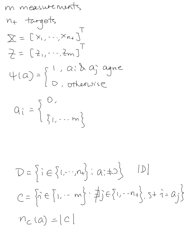
- $m$ measurements, $n_t$ targets, both stacked into vectors: $\ub{X} = [\boldsymbol{x}_1,\dots,\boldsymbol{x}_{n_t}]^{\mathsf T}$, $\;Z = [\boldsymbol{z}_1,\dots,\boldsymbol{z}_m]^{\mathsf T}$.
- Target-oriented association: each target picks a measurement or none, $$a_i \in \{0\} \cup \{1,\dots,m\}, \qquad a_i = 0 \;\text{meaning “missed detection”.}$$
- Consistency indicator (no two targets may claim the same nonzero measurement): $$\psi(\boldsymbol{a}) = \begin{cases} 1, & a_i \neq a_j\ \text{whenever } i\neq j\ \text{and }a_i,a_j\neq0,\\ 0, & \text{otherwise.}\end{cases}$$
- Detected set and clutter set, both functions of $\boldsymbol{a}$: $$\mathcal{D} = \bigl\{ i \in \{1,\dots,n_t\} : a_i \neq 0 \bigr\},\qquad \mathcal{C} = \bigl\{ i \in \{1,\dots,m\} : \nexists\, j \in \{1,\dots,n_t\} \text{ s.t. } i = a_j \bigr\}, \qquad n_c(\boldsymbol{a}) = |\mathcal{C}|.$$
Factorization
Chain rule with the standard structure:
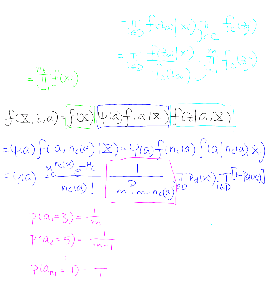
Prior. Targets are independent a priori: $f(\ub{X}) = \prod_{i=1}^{n_t} f(\boldsymbol{x}_i)$.
Measurement term. Measurements claimed by targets follow the measurement model; the rest are clutter with density $f_c$. Multiplying and dividing by $f_c$ over the detected set turns the clutter product into a constant over all $m$ measurements:
$$ f(Z\mid \boldsymbol{a},\ub{X}) = \prod_{i\in\mathcal{D}} f(\boldsymbol{z}_{a_i}\mid\boldsymbol{x}_i) \prod_{j\in\mathcal{C}} f_c(\boldsymbol{z}_j) = \Biggl[\prod_{i\in\mathcal{D}} \frac{f(\boldsymbol{z}_{a_i}\mid\boldsymbol{x}_i)}{f_c(\boldsymbol{z}_{a_i})}\Biggr] \prod_{j=1}^{m} f_c(\boldsymbol{z}_j). $$Association term. Since $n_c(\boldsymbol{a})$ is a function of $\boldsymbol{a}$, we can insert it for free and peel it off with the chain rule. The clutter count is Poisson with mean $\mu_c$; given the counts, all consistent assignments are equally likely:
$$ \psi(\boldsymbol{a})\,f(\boldsymbol{a}\mid\ub{X}) = \psi(\boldsymbol{a})\, f\bigl(\boldsymbol{a}, n_c(\boldsymbol{a})\mid\ub{X}\bigr) = \psi(\boldsymbol{a})\, f\bigl(n_c(\boldsymbol{a})\bigr)\, f\bigl(\boldsymbol{a}\mid n_c(\boldsymbol{a}), \ub{X}\bigr) $$ $$ = \psi(\boldsymbol{a})\; \frac{\mu_c^{\,n_c(\boldsymbol{a})} e^{-\mu_c}}{n_c(\boldsymbol{a})!}\; \frac{1}{{}_{m}P_{\,m-n_c(\boldsymbol{a})}}\; \prod_{i\in\mathcal{D}} P_d(\boldsymbol{x}_i) \prod_{i\notin\mathcal{D}} \bigl[1 - P_d(\boldsymbol{x}_i)\bigr]. $$Combine and drop constants. Writing $\mu_c^{\,n_c} = \mu_c^{\,m} \big/ \mu_c^{\,|\mathcal{D}|}$ pushes one factor $\mu_c$ into the denominator of each detected target's likelihood ratio; the leftovers $\frac{\mu_c^m e^{-\mu_c}}{m!} \prod_{j=1}^m f_c(\boldsymbol{z}_j)$ are constant in $(\ub{X}, \boldsymbol{a})$:
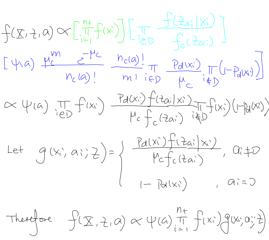
$$ f(\ub{X}, Z, \boldsymbol{a}) \;\propto\; \psi(\boldsymbol{a}) \prod_{i\in\mathcal{D}} f(\boldsymbol{x}_i)\, \frac{P_d(\boldsymbol{x}_i)\, f(\boldsymbol{z}_{a_i}\mid\boldsymbol{x}_i)}{\mu_c\, f_c(\boldsymbol{z}_{a_i})} \prod_{i\notin\mathcal{D}} f(\boldsymbol{x}_i)\bigl(1 - P_d(\boldsymbol{x}_i)\bigr). $$Local likelihood factor. Define
$$ g(\boldsymbol{x}_i, a_i; Z) = \begin{cases} \dfrac{P_d(\boldsymbol{x}_i)\, f(\boldsymbol{z}_{a_i}\mid \boldsymbol{x}_i)}{\mu_c\, f_c(\boldsymbol{z}_{a_i})}, & a_i \neq 0,\\[10px] 1 - P_d(\boldsymbol{x}_i), & a_i = 0. \end{cases} $$Result — scenario 1
$$ f(\ub{X}, Z, \boldsymbol{a}) \;\propto\; \psi(\boldsymbol{a}) \prod_{i=1}^{n_t} f(\boldsymbol{x}_i)\, g(\boldsymbol{x}_i, a_i; Z) $$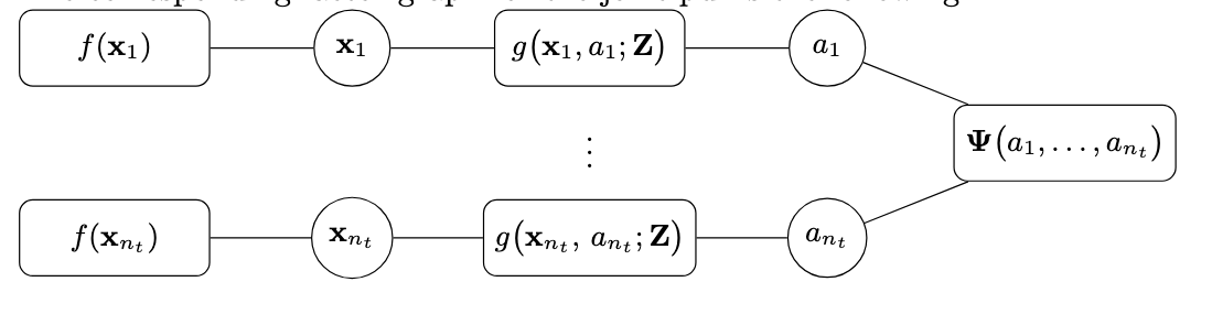
Original handwritten pages (scenario 1)
Point objects, unknown and varying number
Setup
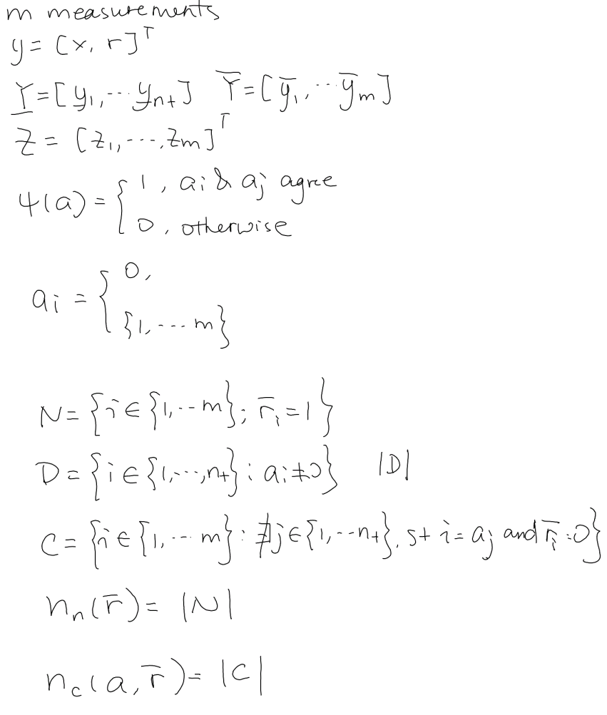
Each object state is augmented with a Bernoulli existence variable, $\boldsymbol{y} = [\boldsymbol{x}, r]^{\mathsf T}$, and every measurement is allowed to start a new potential object:
- Legacy potential objects $\ub{Y} = [\ub{y}_1,\dots,\ub{y}_{n_t}]$ and new potential objects $\ob{Y} = [\ob{y}_1,\dots,\ob{y}_m]$ — one per measurement, with existence indicator $\bar r_i$.
- $Z = [\boldsymbol{z}_1,\dots,\boldsymbol{z}_m]^{\mathsf T}$; association $a_i$ and consistency $\psi(\boldsymbol{a})$ exactly as in scenario 1.
- New-object set, detected set, clutter set — all functions of $(\boldsymbol{a}, \bar{\boldsymbol r})$: $$\mathcal{N} = \{ i \in \{1,\dots,m\} : \bar r_i = 1 \},\qquad n_n(\bar{\boldsymbol r}) = |\mathcal{N}|,$$ $$\mathcal{D} = \{ i : a_i \neq 0 \},\qquad \mathcal{C} = \{ i \in \{1,\dots,m\} : (\nexists\, j \text{ s.t. } i = a_j)\ \land\ \bar r_i = 0 \},\qquad n_c(\boldsymbol{a},\bar{\boldsymbol r}) = |\mathcal{C}|.$$
Factorization
Prior. $f(\ub{Y}) = \prod_{i=1}^{n_t} f(\ub{y}_i)$.
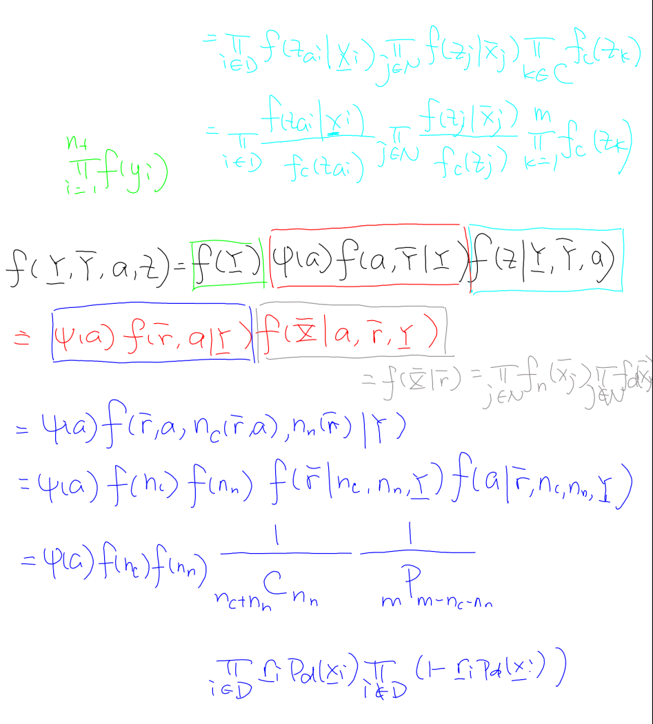
Measurement term. Three kinds of measurements now: claimed by a legacy target, generated by a new object, or clutter. The same multiply-and-divide trick applies:
$$ f(Z\mid\cdot) = \prod_{i\in\mathcal{D}} f(\boldsymbol{z}_{a_i}\mid\ub{x}_i) \prod_{j\in\mathcal{N}} f(\boldsymbol{z}_j\mid\bar{\boldsymbol x}_j) \prod_{k\in\mathcal{C}} f_c(\boldsymbol{z}_k) = \prod_{i\in\mathcal{D}} \frac{f(\boldsymbol{z}_{a_i}\mid\ub{x}_i)}{f_c(\boldsymbol{z}_{a_i})} \prod_{j\in\mathcal{N}} \frac{f(\boldsymbol{z}_j\mid\bar{\boldsymbol x}_j)}{f_c(\boldsymbol{z}_j)} \prod_{k=1}^{m} f_c(\boldsymbol{z}_k). $$New-object states. Conditioned on the existence pattern, non-existent new objects take a dummy density $f_d$: $f(\ob{X}\mid \bar{\boldsymbol r}) = \prod_{j\in\mathcal{N}} f_n(\bar{\boldsymbol x}_j) \prod_{j\notin\mathcal{N}} f_d(\bar{\boldsymbol x}_j)$.
Association term. Both counts are inserted as functions of the random variables and peeled off; $n_c$ and $n_n$ get independent Poisson priors ($\mu_c$, $\mu_n$); given the counts, the split of the $n_c + n_n$ unclaimed measurements into new objects vs clutter is uniform over $\binom{n_c+n_n}{n_n}$ choices, and the assignment of detected targets to measurements is uniform over ${}_{m}P_{\,m-n_c-n_n} = m!/(n_c+n_n)!$ ordered choices:
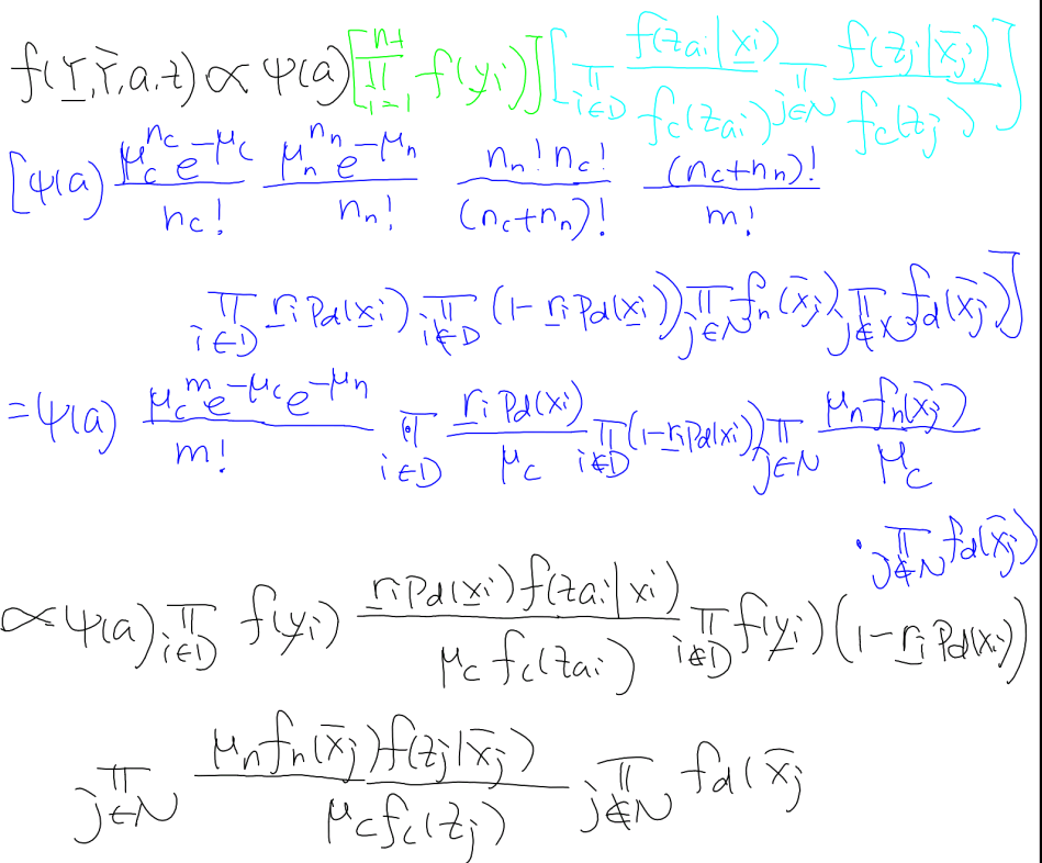
$$ \psi(\boldsymbol{a})\, f(\bar{\boldsymbol r}, \boldsymbol{a}\mid\ub{Y}) = \psi(\boldsymbol{a})\, f\bigl(\bar{\boldsymbol r}, \boldsymbol{a}, n_c(\bar{\boldsymbol r},\boldsymbol{a}), n_n(\bar{\boldsymbol r})\mid\ub{Y}\bigr) = \psi(\boldsymbol{a})\, f(n_c)\, f(n_n)\, f(\bar{\boldsymbol r}\mid n_c, n_n, \ub{Y})\, f(\boldsymbol{a}\mid \bar{\boldsymbol r}, n_c, n_n, \ub{Y}) $$ $$ = \psi(\boldsymbol{a})\, f(n_c)\, f(n_n)\; \frac{1}{\binom{n_c+n_n}{n_n}}\; \frac{1}{{}_{m}P_{\,m-n_c-n_n}}\; \prod_{i\in\mathcal{D}} \ub{r}_i P_d(\ub{x}_i) \prod_{i\notin\mathcal{D}} \bigl(1 - \ub{r}_i P_d(\ub{x}_i)\bigr). $$Combine and drop constants. The binomial and permutation denominators merge into $\frac{n_n!\, n_c!}{(n_c+n_n)!}\cdot\frac{(n_c+n_n)!}{m!} = \frac{n_n!\, n_c!}{m!}$, the Poisson factorials cancel, and $\mu_c^{\,n_c} = \mu_c^m / \mu_c^{\,|\mathcal{D}| + n_n}$ distributes one $\mu_c$ under every likelihood ratio:
$$ f(\ub{Y}, \ob{Y}, \boldsymbol{a}, Z) \;\propto\; \psi(\boldsymbol{a}) \prod_{i\in\mathcal{D}} f(\ub{y}_i)\, \frac{\ub{r}_i P_d(\ub{x}_i)\, f(\boldsymbol{z}_{a_i}\mid\ub{x}_i)}{\mu_c\, f_c(\boldsymbol{z}_{a_i})} \prod_{i\notin\mathcal{D}} f(\ub{y}_i)\bigl(1 - \ub{r}_i P_d(\ub{x}_i)\bigr)\; \prod_{j\in\mathcal{N}} \frac{\mu_n f_n(\bar{\boldsymbol x}_j)\, f(\boldsymbol{z}_j\mid\bar{\boldsymbol x}_j)}{\mu_c\, f_c(\boldsymbol{z}_j)} \prod_{j\notin\mathcal{N}} f_d(\bar{\boldsymbol x}_j). $$Local likelihood factors. For legacy potential objects ($\ub{r}_i = 0$ means the object does not exist, so it cannot be detected):
$$ \ub{g}(\ub{x}_i, \ub{r}_i, a_i; Z) = \begin{cases} \dfrac{P_d(\ub{x}_i)\, f(\boldsymbol{z}_{a_i}\mid\ub{x}_i)}{\mu_c\, f_c(\boldsymbol{z}_{a_i})}, & i \in \mathcal{D},\ \ub{r}_i = 1,\\[10px] 1 - P_d(\ub{x}_i), & i \notin \mathcal{D},\ \ub{r}_i = 1,\\[4px] 0, & i \in \mathcal{D},\ \ub{r}_i = 0,\\[4px] 1, & i \notin \mathcal{D},\ \ub{r}_i = 0. \end{cases} $$For new potential objects, let $\mathcal{T} = \{ i \in \{1,\dots,m\} : \exists\, j \text{ s.t. } a_j = i \}$ be the measurements already claimed by legacy targets — a claimed measurement cannot also start a new object:
$$ \bar{g}(\bar{\boldsymbol x}_i, \bar r_i, \boldsymbol{a}; \boldsymbol{z}_i) = \begin{cases} \dfrac{\mu_n f_n(\bar{\boldsymbol x}_i)\,f(\boldsymbol{z}_i\mid\bar{\boldsymbol x}_i)}{\mu_c\, f_c(\boldsymbol{z}_i)}, & i \notin \mathcal{T},\ \bar r_i = 1,\\[10px] 0, & i \in \mathcal{T},\ \bar r_i = 1,\\[4px] f_d(\bar{\boldsymbol x}_i), & \bar r_i = 0. \end{cases} $$Result — scenario 2
$$ f(\ub{Y}, \ob{Y}, \boldsymbol{a}, Z) \;\propto\; \psi(\boldsymbol{a}) \prod_{i=1}^{n_t} f(\ub{y}_i)\, \ub{g}(\ub{y}_i, a_i; Z) \prod_{j=1}^{m} \bar{g}(\ob{y}_j, \boldsymbol{a}; \boldsymbol{z}_j) $$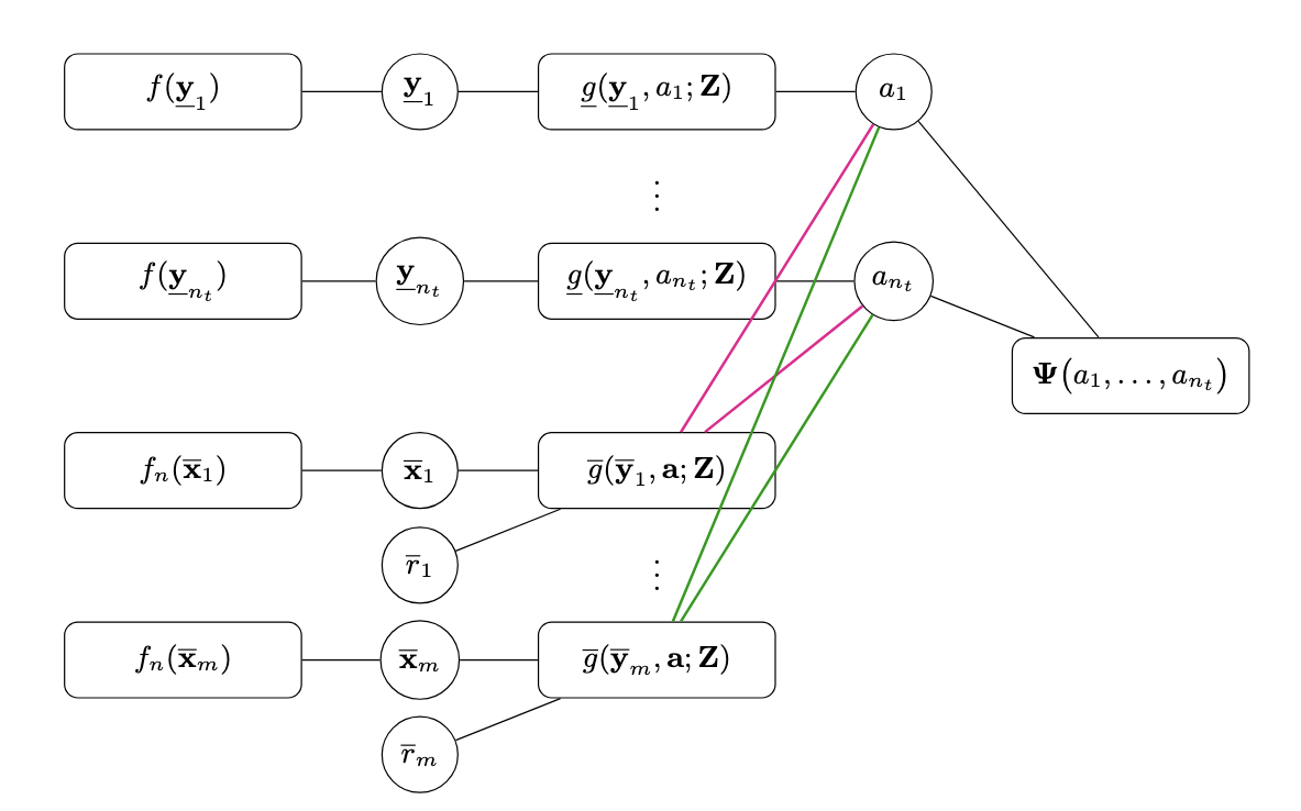
Original handwritten pages (scenario 2)
Extended objects, known and constant number
Setup
An extended object can generate several measurements per scan, so the association is now measurement-oriented: each measurement points at its source. The state carries an extent, $\boldsymbol{y} = [\boldsymbol{x}, \boldsymbol{e}]^{\mathsf T}$.
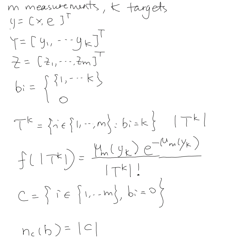
- $m$ measurements, $K$ objects: $Y = [\boldsymbol{y}_1,\dots,\boldsymbol{y}_K]^{\mathsf T}$, $Z = [\boldsymbol{z}_1,\dots,\boldsymbol{z}_m]^{\mathsf T}$.
- Association per measurement: $b_i \in \{1,\dots,K\} \cup \{0\}$, with $b_i = 0$ meaning clutter. No consistency factor $\psi$ is needed — a measurement has exactly one source by construction.
- Measurement cell of object $k$ and clutter set: $$\mathcal{T}^k = \{ i \in \{1,\dots,m\} : b_i = k \},\qquad \mathcal{C} = \{ i : b_i = 0 \},\qquad n_c(\boldsymbol{b}) = |\mathcal{C}|.$$
- The number of measurements an object generates is Poisson with a state-dependent rate: $$f\bigl(|\mathcal{T}^k|\bigr) = \frac{\mu_m(\boldsymbol{y}_k)^{|\mathcal{T}^k|}\, e^{-\mu_m(\boldsymbol{y}_k)}}{|\mathcal{T}^k|!}.$$
Factorization
Prior. $f(Y) = \prod_{k=1}^{K} f(\boldsymbol{y}_k)$.
Measurement term.
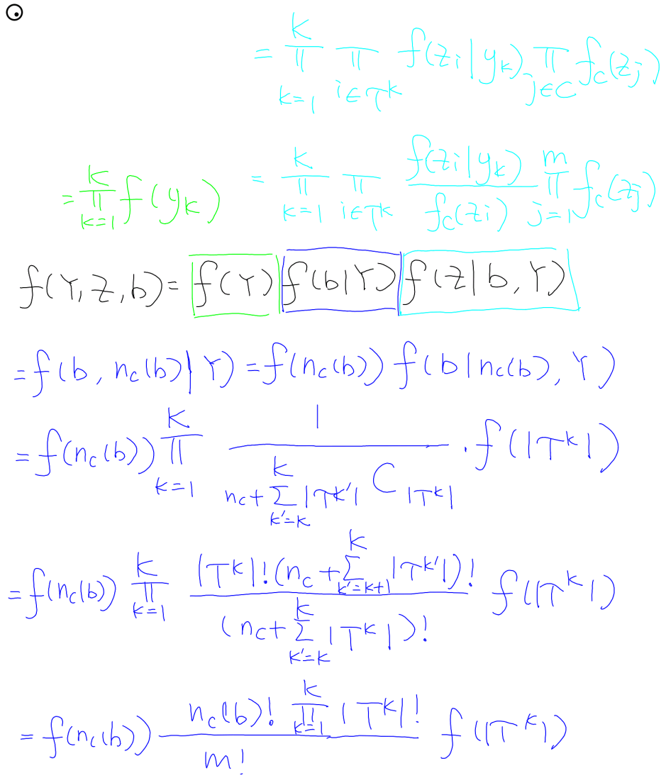
$$ f(Z\mid \boldsymbol{b}, Y) = \prod_{k=1}^{K} \prod_{i\in\mathcal{T}^k} f(\boldsymbol{z}_i\mid\boldsymbol{y}_k) \prod_{j\in\mathcal{C}} f_c(\boldsymbol{z}_j) = \Biggl[\prod_{k=1}^{K} \prod_{i\in\mathcal{T}^k} \frac{f(\boldsymbol{z}_i\mid\boldsymbol{y}_k)}{f_c(\boldsymbol{z}_i)}\Biggr] \prod_{j=1}^{m} f_c(\boldsymbol{z}_j). $$Association term. Insert $n_c(\boldsymbol{b})$, then draw the cells one object at a time: object $k$ chooses which $|\mathcal{T}^k|$ of the still-unassigned $n_c + \sum_{k'=k}^{K}|\mathcal{T}^{k'}|$ measurements are its own, uniformly:
$$ f(\boldsymbol{b}\mid Y) = f\bigl(n_c(\boldsymbol{b})\bigr)\, f\bigl(\boldsymbol{b}\mid n_c(\boldsymbol{b}), Y\bigr) = f\bigl(n_c(\boldsymbol{b})\bigr) \prod_{k=1}^{K} \binom{n_c + \sum_{k'=k}^{K}|\mathcal{T}^{k'}|}{|\mathcal{T}^{k}|}^{-1} f\bigl(|\mathcal{T}^k|\bigr). $$The product of inverse binomials telescopes:
$$ \prod_{k=1}^{K} \frac{|\mathcal{T}^k|!\,\bigl(n_c + \sum_{k'=k+1}^{K}|\mathcal{T}^{k'}|\bigr)!}{\bigl(n_c + \sum_{k'=k}^{K}|\mathcal{T}^{k'}|\bigr)!} = \frac{n_c(\boldsymbol{b})!\,\prod_{k=1}^{K} |\mathcal{T}^k|!}{m!}, $$so that
$$ f(\boldsymbol{b}\mid Y) = f\bigl(n_c(\boldsymbol{b})\bigr)\; \frac{n_c(\boldsymbol{b})!\,\prod_{k=1}^{K}|\mathcal{T}^k|!}{m!}\; \prod_{k=1}^{K} f\bigl(|\mathcal{T}^k|\bigr). $$Combine and drop constants. The cell-size factorials cancel against the Poisson PMFs, $\mu_c^{\,n_c} = \mu_c^m \big/ \prod_k \mu_c^{|\mathcal{T}^k|}$ places one $\mu_c$ under each per-measurement ratio, and $\frac{\mu_c^m e^{-\mu_c}}{m!}\prod_j f_c(\boldsymbol{z}_j)$ is constant:
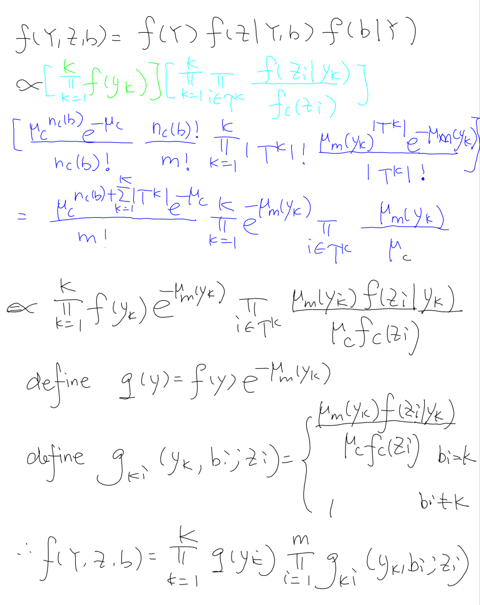
$$ f(Y, Z, \boldsymbol{b}) \;\propto\; \prod_{k=1}^{K} f(\boldsymbol{y}_k)\, e^{-\mu_m(\boldsymbol{y}_k)} \prod_{i\in\mathcal{T}^k} \frac{\mu_m(\boldsymbol{y}_k)\, f(\boldsymbol{z}_i\mid\boldsymbol{y}_k)}{\mu_c\, f_c(\boldsymbol{z}_i)}. $$Local factors. Define the modified prior and the pairwise factors
$$ g(\boldsymbol{y}_k) = f(\boldsymbol{y}_k)\, e^{-\mu_m(\boldsymbol{y}_k)}, \qquad g_{ki}(\boldsymbol{y}_k, b_i; \boldsymbol{z}_i) = \begin{cases} \dfrac{\mu_m(\boldsymbol{y}_k)\, f(\boldsymbol{z}_i\mid\boldsymbol{y}_k)}{\mu_c\, f_c(\boldsymbol{z}_i)}, & b_i = k,\\[10px] 1, & b_i \neq k. \end{cases} $$Result — scenario 3
$$ f(Y, Z, \boldsymbol{b}) \;\propto\; \prod_{k=1}^{K}\!\left[g(\boldsymbol{y}_k) \prod_{i=1}^{m} g_{ki}(\boldsymbol{y}_k, b_i; \boldsymbol{z}_i)\right] $$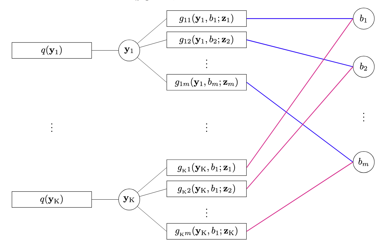
Original handwritten pages (scenario 3)
Extended objects, unknown and varying number
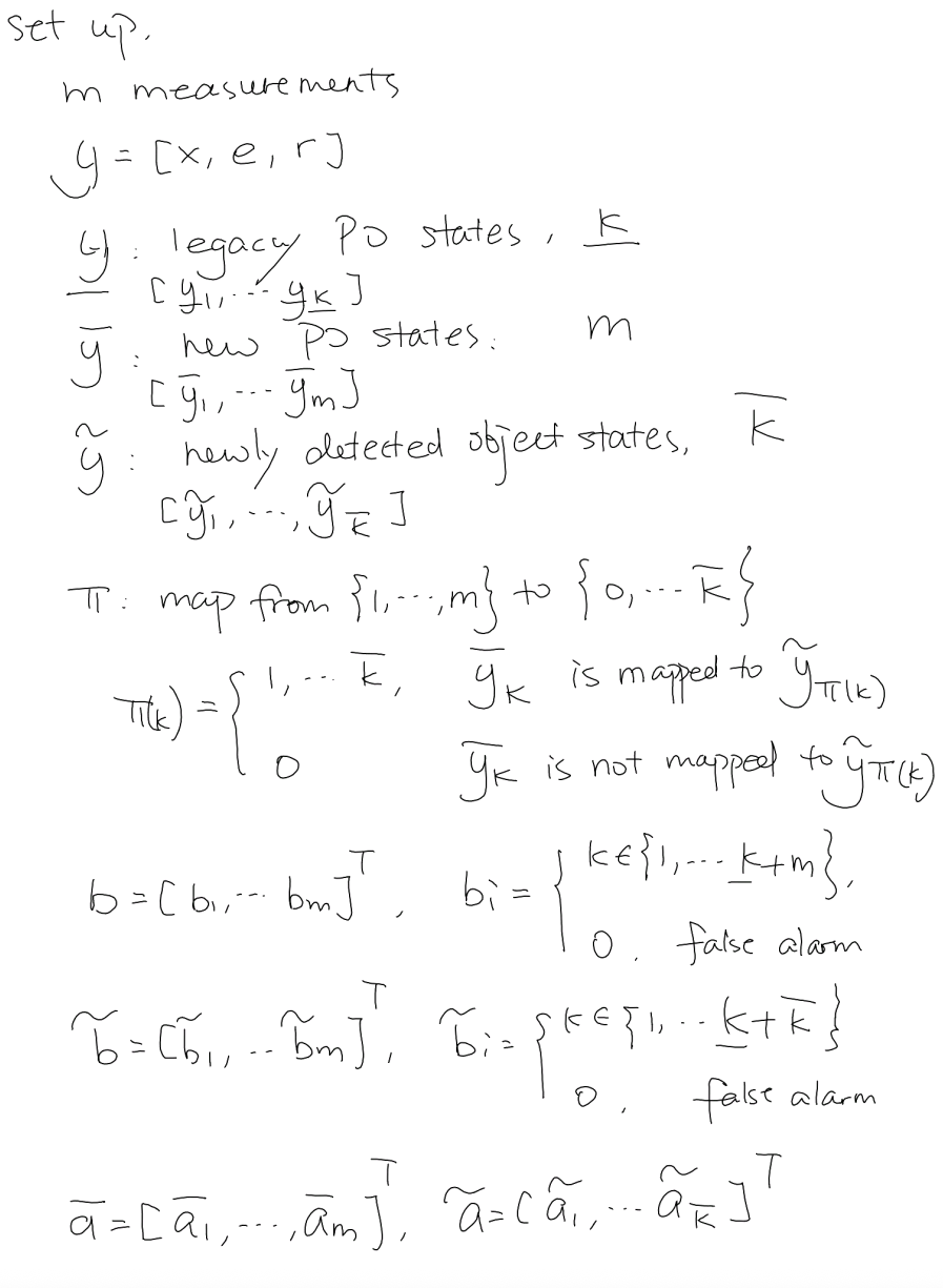
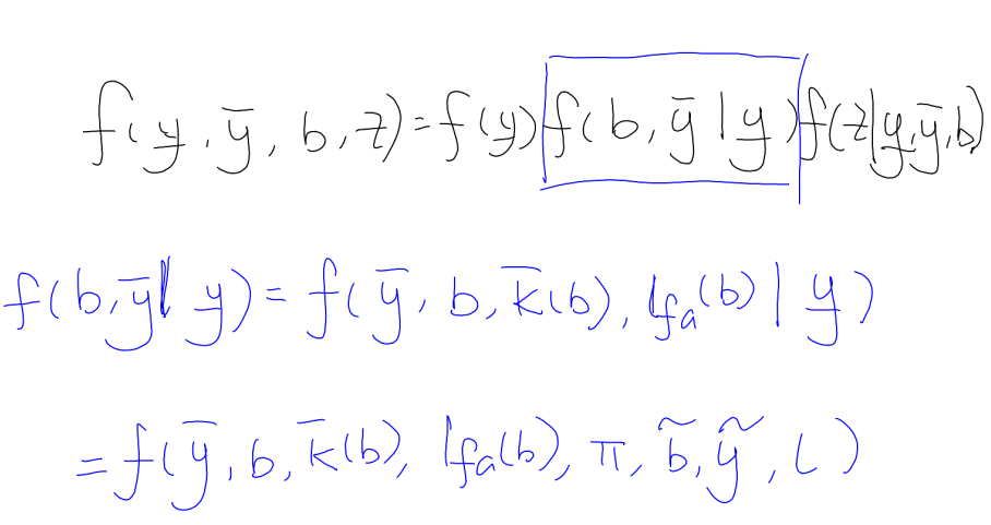
The hardest case, following the construction of Meyer & Williams [3]: extended objects with existence variables, measurement-oriented association, and new objects spawned from measurements. The trick is to introduce a redundant set of auxiliary variables (the newly detected objects and a mapping onto them), derive the joint in that over-complete representation where every conditional is simple, and then marginalize the auxiliaries back out.
Setup
- $M$ measurements; augmented state $\boldsymbol{y} = [\boldsymbol{x}, \boldsymbol{e}, r]$ (kinematics, extent, existence).
- Legacy potential objects $\ub{y}_1,\dots,\ub{y}_{\underline K}$ ($\underline K$ of them); new potential objects $\ob{y}_1,\dots,\ob{y}_M$ (one per measurement); newly detected objects $\tb{y}_1,\dots,\tb{y}_{\overline K}$ ($\overline K$ of them — auxiliary, to be integrated out).
- Mapping $\pi : \{1,\dots,M\} \to \{0,\dots,\overline K\}$: $\pi(k) \in \{1,\dots,\overline K\}$ if new PO $\ob{y}_k$ corresponds to newly detected object $\tb{y}_{\pi(k)}$, and $\pi(k)=0$ otherwise.
- Two association vectors: $$\boldsymbol{b} = [b_1,\dots,b_M]^{\mathsf T},\quad b_i \in \{0,1,\dots,\underline K + i\}, \qquad \tb{b} = [\tilde b_1,\dots,\tilde b_M]^{\mathsf T},\quad \tilde b_i \in \{1,\dots,\underline K + \overline K\} \cup \{0\},$$ with $0$ meaning false alarm; and measurement lists $\ob{a} = [\bar a_1,\dots,\bar a_M]^{\mathsf T}$, $\tb{a} = [\tilde a_1,\dots,\tilde a_{\overline K}]^{\mathsf T}$.
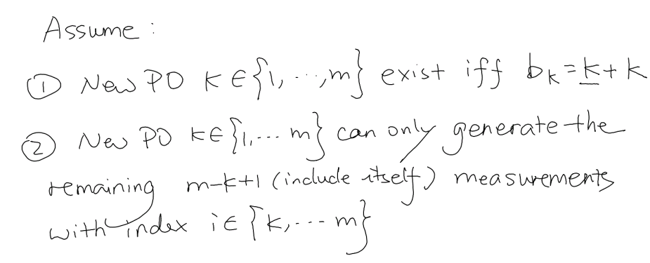
- Assumptions that make $\boldsymbol{b}$ well defined:
- new PO $k \in \{1,\dots,M\}$ exists iff $b_k = \underline K + k$ (a new object is anchored to the first measurement it generates);
- new PO $k$ can only generate the remaining $M - k + 1$ measurements (including its own), i.e. those with index $i \in \{k,\dots,M\}$.
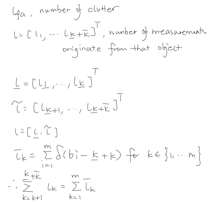
- Counts, all functions of the association: $l_{\mathrm{fa}}$ = number of false alarms; $\boldsymbol{l} = [l_1,\dots,l_{\underline K + \overline K}]^{\mathsf T}$ = number of measurements from each object, split as $\ub{l} = [l_1,\dots,l_{\underline K}]^{\mathsf T}$ (legacy) and $\tb{l} = [l_{\underline K + 1},\dots,l_{\underline K + \overline K}]^{\mathsf T}$ (newly detected); and per new PO $$\bar l_k = \sum_{i=1}^{M} \delta\bigl(b_i - (\underline K + k)\bigr),\ k \in \{1,\dots,M\} \qquad\Longrightarrow\qquad \sum_{k=\underline K+1}^{\underline K + \overline K} l_k = \sum_{k=1}^{M} \bar l_k.$$
- $\mathcal{D}_{\ub{y}}$ denotes the existing legacy objects ($\ub{r}_k = 1$) and $\mathcal{D}_{\boldsymbol{b}}$ the new POs that exist ($b_k = \underline K + k$).
Step 1 — chain-rule expansion in the over-complete representation
where the second line drops every variable that each conditional does not actually depend on. Each factor now has a simple closed form.
Measurement counts. A newly detected object was detected, so its count is a zero-truncated Poisson; existing legacy objects have ordinary Poisson counts; non-existing legacy objects generate nothing ($p(\boldsymbol{l}\mid\cdot)$ factorizes as $p(\tb{l}\mid \overline K, \tb{y})\, p(\ub{l}\mid \ub{y})$):
$$ p(\boldsymbol{l} \mid \overline K, \tb{y}, \ub{y}) = \Biggl(\prod_{k=1}^{\overline K} \frac{\mu_m(\tb{x}_k, \tb{e}_k)^{\tilde l_k}}{\tilde l_k!}\, \frac{e^{-\mu_m(\tb{x}_k, \tb{e}_k)}}{1 - e^{-\mu_m(\tb{x}_k, \tb{e}_k)}}\Biggr) \Biggl(\prod_{k\in\mathcal{D}_{\ub{y}}} \frac{\mu_m(\ub{x}_k, \ub{e}_k)^{l_k}}{l_k!}\, e^{-\mu_m(\ub{x}_k, \ub{e}_k)}\Biggr) \prod_{k\notin\mathcal{D}_{\ub{y}}} \delta(l_k). $$Association given counts. Uniform over all assignments consistent with the cell sizes; the telescoping-binomial identity from scenario 3 gives
$$ p(\tb{b} \mid \boldsymbol{l}, l_{\mathrm{fa}}) = \frac{l_{\mathrm{fa}}!\,\Bigl(\prod_{k=1}^{\underline K + \overline K} l_k!\Bigr)} {\Bigl(l_{\mathrm{fa}} + \sum_{k=1}^{\underline K + \overline K} l_k\Bigr)!}\,, \qquad\text{via}\qquad \prod_{k=1}^{\underline K+\overline K}\binom{l_{\mathrm{fa}} + \sum_{k'=k}^{\underline K+\overline K} l_{k'}}{l_k} = \frac{\bigl(l_{\mathrm{fa}} + \sum_{k=1}^{\underline K+\overline K} l_k\bigr)!} {l_{\mathrm{fa}}!\,\bigl(\prod_{k=1}^{\underline K+\overline K} l_k!\bigr)}\,. $$Mapping. Given $\tb{b}$, the mapping is deterministic: $p(\boldsymbol{\pi} \mid \tb{b}) = \delta(\boldsymbol{\pi} - \boldsymbol{\pi}_{\tb{b}})$.
New POs given the mapping. A new PO that is mapped copies the state and measurement list of its newly detected object; an unmapped one does not exist:
$$ f(\ob{y}, \boldsymbol{b} \mid \tb{b}, \tb{y}, \boldsymbol{\pi}) = \Biggl(\prod_{\substack{k=1\\ \pi(k) \gt 0}}^{M} \bar r_k\, \delta\bigl(\ob{y}_k - \tb{y}_{\pi(k)}\bigr)\, \delta\bigl(\ob{a}_k - \tb{a}_{\pi(k)}\bigr)\Biggr) \prod_{\substack{k=1\\ \pi(k)=0}}^{M} f_d(\ob{x}_k, \ob{e}_k)\,(1 - \bar r_k)\, \delta\bigl(\lVert\ob{a}_k\rVert_1\bigr). $$Priors.
$$ p(l_{\mathrm{fa}}) = \frac{\mu_{\mathrm{fa}}^{\,l_{\mathrm{fa}}}}{l_{\mathrm{fa}}!}\, e^{-\mu_{\mathrm{fa}}}, \qquad f(\tb{y} \mid \overline K) = \prod_{k=1}^{\overline K} \tilde r_k\, f_n(\tb{x}_k, \tb{e}_k), \qquad p(\overline K) = \frac{\mu_n^{\,\overline K}}{\overline K!}\, e^{-\mu_n}. $$Step 2 — marginalize the newly detected states $\tb{y}$
Substituting all factors and integrating $\tb{y}$ out — the delta functions $\delta(\ob{y}_k - \tb{y}_{\pi(k)})$ simply transfer each newly detected state onto its new PO:
$$ f(\ob{y}, \boldsymbol{b}, \tb{b}, \boldsymbol{\pi}, \overline K, l_{\mathrm{fa}} \mid \ub{y}) = \int f(\ob{y}, \tb{y}, \boldsymbol{b}, \tb{b}, \boldsymbol{\pi}, \overline K, l_{\mathrm{fa}} \mid \ub{y})\, \mathrm{d}\tb{y} = f(\ob{y}, \boldsymbol{b}, \tb{b} \mid \overline K, \ub{y}, l_{\mathrm{fa}}, \boldsymbol{\pi})\, p(\boldsymbol{\pi}\mid\tb{b})\, p(\overline K)\, p(l_{\mathrm{fa}}) $$with
$$ \begin{aligned} f(\ob{y}, \boldsymbol{b}, \tb{b} \mid \overline K, \ub{y}, l_{\mathrm{fa}}, \boldsymbol{\pi}) ={}& \Biggl(\prod_{\substack{k=1\\ \pi(k) \gt 0}}^{M} \bar r_k\, \frac{\mu_m(\ob{x}_k, \ob{e}_k)^{\tilde l_{\pi(k)}}}{\tilde l_{\pi(k)}!}\, \frac{e^{-\mu_m(\ob{x}_k, \ob{e}_k)}}{1 - e^{-\mu_m(\ob{x}_k, \ob{e}_k)}}\, f_n(\ob{x}_k, \ob{e}_k)\, \delta\bigl(\ob{a}_k - \tb{a}_{\pi(k)}\bigr)\Biggr)\\[2px] &\times \Biggl(\prod_{k\in\mathcal{D}_{\ub{y}}} \frac{\mu_m(\ub{x}_k, \ub{e}_k)^{l_k}}{l_k!}\, e^{-\mu_m(\ub{x}_k, \ub{e}_k)}\Biggr) \Biggl(\prod_{k\notin\mathcal{D}_{\ub{y}}} \delta(l_k)\Biggr) \Biggl(\prod_{\substack{k=1\\ \pi(k)=0}}^{M} f_d(\ob{x}_k, \ob{e}_k)(1 - \bar r_k)\, \delta\bigl(\lVert\ob{a}_k\rVert_1\bigr)\Biggr)\\[2px] &\times \frac{l_{\mathrm{fa}}!\,\Bigl(\prod_{k=1}^{\underline K + \overline K} l_k!\Bigr)} {\Bigl(l_{\mathrm{fa}} + \sum_{k=1}^{\underline K + \overline K} l_k\Bigr)!}\,. \end{aligned} $$Step 3 — sum out the auxiliary association $\tb{b}$ (and $\boldsymbol{\pi}$)
$\boldsymbol{\pi}$ collapses by the delta $p(\boldsymbol{\pi}\mid\tb{b}) = \delta(\boldsymbol{\pi} - \boldsymbol{\pi}_{\tb{b}})$, leaving a sum over $\tb{b}$:
$$ f(\ob{y}, \boldsymbol{b}, \overline K, l_{\mathrm{fa}} \mid \ub{y}) = p(\overline K)\, p(l_{\mathrm{fa}}) \sum_{\tb{b}} f\bigl(\ob{y}, \boldsymbol{b}, \tb{b} \mid \overline K, \ub{y}, l_{\mathrm{fa}}, \boldsymbol{\pi}_{\tb{b}}\bigr). $$Every relabeling of the $\overline K$ newly detected objects produces the same $(\ob{y}, \boldsymbol{b})$, so the sum contributes a factor $\overline K!$ and converts $\tilde l_{\pi(k)} \to \bar l_k$, $\mathcal{T}$-indexed products into $\mathcal{D}_{\boldsymbol{b}}$-indexed ones:
$$ \begin{aligned} f(\ob{y}, \boldsymbol{b}, \overline K, l_{\mathrm{fa}} \mid \ub{y}) ={}& p(\overline K)\, p(l_{\mathrm{fa}})\, \frac{\overline K!\; l_{\mathrm{fa}}!\,\Bigl(\prod_{k=1}^{\underline K} l_k!\Bigr)\Bigl(\prod_{k=1}^{M} \bar l_k!\Bigr)} {\Bigl(l_{\mathrm{fa}} + \sum_{k=1}^{\underline K} l_k + \sum_{k'=1}^{M} \bar l_{k'}\Bigr)!} \Biggl(\prod_{k\in\mathcal{D}_{\ub{y}}} \frac{\mu_m(\ub{x}_k, \ub{e}_k)^{l_k}}{l_k!}\, e^{-\mu_m(\ub{x}_k, \ub{e}_k)}\Biggr) \Biggl(\prod_{k\notin\mathcal{D}_{\ub{y}}} \delta(l_k)\Biggr)\\[2px] &\times \Biggl(\prod_{k\in\mathcal{D}_{\boldsymbol{b}}} \bar r_k\, \frac{\mu_m(\ob{x}_k, \ob{e}_k)^{\bar l_k}}{\bar l_k!}\, \frac{e^{-\mu_m(\ob{x}_k, \ob{e}_k)}}{1 - e^{-\mu_m(\ob{x}_k, \ob{e}_k)}}\, f_n(\ob{x}_k, \ob{e}_k)\Biggr) \prod_{k\notin\mathcal{D}_{\boldsymbol{b}}} f_d(\ob{x}_k, \ob{e}_k)(1 - \bar r_k)\, \delta(\bar l_k). \end{aligned} $$Substituting the Poisson priors $p(\overline K)$ and $p(l_{\mathrm{fa}})$ — their factorials $\overline K!$ and $l_{\mathrm{fa}}!$ cancel exactly, $|\mathcal{D}_{\boldsymbol{b}}| = \overline K$ and $l_{\mathrm{fa}} = M - \sum_k l_k - \sum_{k'} \bar l_{k'}$ — gives the conditional prior over new POs, associations, and the measurement count. The measurement values $Z$ have not yet entered:
Conditional-prior result — scenario 4
$$ \begin{aligned} f(\ob{y}, \boldsymbol{b}, M \mid \ub{y}) ={}& \Biggl(\prod_{k\in\mathcal{D}_{\boldsymbol{b}}} \bar r_k\, f_n(\ob{x}_k, \ob{e}_k)\, \mu_m(\ob{x}_k, \ob{e}_k)^{\bar l_k}\, \frac{e^{-\mu_m(\ob{x}_k, \ob{e}_k)}}{1 - e^{-\mu_m(\ob{x}_k, \ob{e}_k)}}\Biggr) \Biggl(\prod_{k\notin\mathcal{D}_{\boldsymbol{b}}} (1 - \bar r_k)\, f_d(\ob{x}_k, \ob{e}_k)\, \delta(\bar l_k)\Biggr)\\[2px] &\times \Biggl(\prod_{k\in\mathcal{D}_{\ub{y}}} \mu_m(\ub{x}_k, \ub{e}_k)^{l_k}\, e^{-\mu_m(\ub{x}_k, \ub{e}_k)}\Biggr) \Biggl(\prod_{k\notin\mathcal{D}_{\ub{y}}} \delta(\ub{l}_k)\Biggr)\, \frac{\mu_n^{\,|\mathcal{D}_{\boldsymbol{b}}|}\; \mu_{\mathrm{fa}}^{\,\bigl(M - \sum_{k=1}^{\underline K} l_k - \sum_{k'=1}^{M} \bar l_{k'}\bigr)}\; e^{-(\mu_n + \mu_{\mathrm{fa}})}}{M!}\,. \end{aligned} $$BP-ready potentials
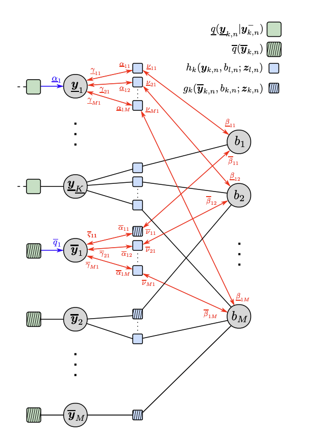
Distributing the counts over per-measurement factors (each power $\mu_m^{\bar l_k}$ or $\mu_m^{l_k}$ becomes one $\mu_m$ per associated measurement, paired with the likelihood ratio) turns the joint into the standard node/edge potentials of the extended-object BP factor graph:
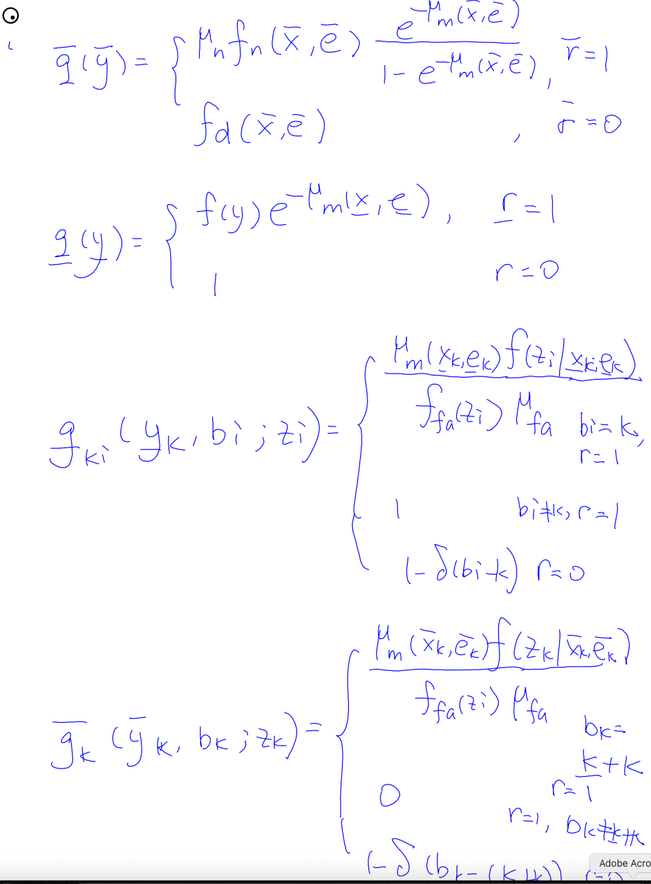
$$ \bar q(\ob{y}) = \begin{cases} \mu_n\, f_n(\ob{x}, \ob{e})\, \dfrac{e^{-\mu_m(\ob{x}, \ob{e})}}{1 - e^{-\mu_m(\ob{x}, \ob{e})}}, & \bar r = 1,\\[10px] f_d(\ob{x}, \ob{e}), & \bar r = 0, \end{cases} \qquad\qquad \underline q(\ub{y}) = \begin{cases} f^{-}(\ub{y})\, e^{-\mu_m(\ub{x}, \ub{e})}, & \ub{r} = 1,\\[6px] f^{-}(\ub{y}), & \ub{r} = 0, \end{cases} $$Here $f^{-}(\ub y)$ is the predicted augmented-state density, including existence mass and the chosen dummy density when $\ub r=0$. In the multi-scan paper, $\underline q$ is the corresponding pseudo-transition factor, not merely a scalar 1 in the non-existing branch.
with pairwise factors for legacy objects ($k \in \{1,\dots,\underline K\}$, measurement $i$):
$$ \underline g_{ki}(\ub{y}_k, b_i; \boldsymbol{z}_i) = \begin{cases} \dfrac{\mu_m(\ub{x}_k, \ub{e}_k)\, f(\boldsymbol{z}_i \mid \ub{x}_k, \ub{e}_k)}{f_{\mathrm{fa}}(\boldsymbol{z}_i)\,\mu_{\mathrm{fa}}}, & b_i = k,\ \ub{r}_k = 1,\\[10px] 1, & b_i \neq k,\ \ub{r}_k = 1,\\[4px] 1 - \delta(b_i - k), & \ub{r}_k = 0, \end{cases} $$and for new potential objects ($k \in \{1,\dots,M\}$):
$$ \bar g_{k}(\ob{y}_k, b_k; \boldsymbol{z}_k) = \begin{cases} \dfrac{\mu_m(\ob{x}_k, \ob{e}_k)\, f(\boldsymbol{z}_k \mid \ob{x}_k, \ob{e}_k)}{f_{\mathrm{fa}}(\boldsymbol{z}_k)\,\mu_{\mathrm{fa}}}, & b_k = \underline K + k,\ \bar r_k = 1,\\[10px] 0, & b_k \neq \underline K + k,\ \bar r_k = 1,\\[4px] 1 - \delta\bigl(b_k - (\underline K + k)\bigr), & \bar r_k = 0. \end{cases} $$For every later measurement $i\in\{k+1,\dots,M\}$, the same new PO also needs a pairwise factor
$$ \bar h_{ki}(\ob{y}_k,b_i;\boldsymbol z_i)= \begin{cases} \dfrac{\mu_m(\ob{x}_k,\ob{e}_k)f(\boldsymbol z_i\mid\ob{x}_k,\ob{e}_k)} {\mu_{\mathrm{fa}}f_{\mathrm{fa}}(\boldsymbol z_i)}, & b_i=\underline K+k,\ \bar r_k=1,\\[10px] 1, & b_i\neq\underline K+k,\ \bar r_k=1,\\[4px] 1-\delta\bigl(b_i-(\underline K+k)\bigr), & \bar r_k=0. \end{cases} $$Thus the single-scan, measurement-conditioned factorization has the structure
Original handwritten pages (scenario 4)
Derivation for GrBP
Eqs. (A.1)–(A.9) · Open these slides →
GrBP provides an alternative for extended objects with an unknown count: precluster the detections, then associate whole groups. The time index is omitted for readability.
$\boldsymbol Z$→Preclustering
$\mathcal P=\mathcal C(\boldsymbol Z)$→Fixed groups
$\boldsymbol Z^G$→Data association
$\boldsymbol a,\boldsymbol b$
A. Notation and setup
There are $n^t$ legacy components and $n^g$ newborn components, one newborn candidate per group, rather than one per raw detection. Each state contains kinematics $\boldsymbol x$, extent $\boldsymbol E$, and existence $r$. A fixed grouping can contain many groups. The one-group special case is $n^g=1$, not $m=1$.
Eq. (A.1) uses the display shorthand $s=(\boldsymbol x,\boldsymbol E)$. The model assumes a product previous posterior and independent transitions to obtain the predicted product prior.
$a^p=j$ means legacy target $p$ generates the whole group $j$. The variable $b^j=p$ records the same event from the group side. Crucially, $b^j=0$ means not generated by a legacy target, so the group may be clutter or a newly detected target.
Each target generates at most one group and each group contains measurements from only one source. The pairwise indicators enforce exclusive legacy associations. The newborn factor below additionally rules out a newborn in a group already claimed by a legacy target. On these feasible hypotheses, define the three count sets:
B. Joint PDF and factorization · Eq. (A.2)
Dependence on the fixed partition $\mathcal P=\mathcal C(\boldsymbol Z)$ is suppressed. This chain-rule structure separates the factors before approximating the association and group-likelihood contributions. The following display shorthands $B$, $L_{\mathrm L}$, $L_{\mathrm N}$, $F_c$, and $R_j$ distinguish the state-density and likelihood factors.
B.1. Count models and factorial cancellation · Eqs. (A.3)–(A.4)
$\mu_g$ is the mean number of clutter groups after preclustering. It is not generally the raw clutter-detection mean $\mu_c$. The parameter $\mu_n$ is the mean number of detected newborns. No undetected-intensity substitution is made in this variant.
Conditioned on the counts, the model uses a uniform choice of newborn groups among the unclaimed groups and a uniform ordered assignment of detected legacy targets:
The product cancels the $n^c!$ and $n^n!$ in the Poisson terms. The remaining denominator is $n^g!$, not $m!$. The newborn state-density contribution is
With those factors, the intermediate association expression is
B.2. Group likelihoods · Eq. (A.5)
A legacy group carries one $e^{-\mu_m(s)}$ for the entire group. A newborn is already detected by assumption, so the model uses the zero-truncated factor $1/[1-e^{-\mu_m(s)}]$. The clutter group is represented by the product of its spatial clutter densities. These conventions use a clutter-group model, not a substituted raw-PPP clutter intensity per point.
B.3. Separate the constant · Eq. (A.6)
For fixed observations and fixed model parameters, $C$ is independent of the target states, existence variables, and associations. It may therefore be removed when normalizing that scan’s posterior. It is not removable without reconsideration when comparing partition hypotheses or estimating $\mu_g$ or $\mu_n$.
B.4. Legacy local factor · Eq. (A.7)
Expanding $R_a(s)$ gives the full legacy factor in Eq. (A.7). The group contributes one $1/\mu_g$, regardless of its size. A null assignment for an existing target has weight $e^{-\mu_m(s)}$. A nonexistent target has weight one only for a null assignment and cannot explain a group.
B.5. Newborn local factor · Eq. (A.8)
Expanding $R_j(s)$ gives the full newborn factor in Eq. (A.8). Both $\mu_n f_n(s)$ and the zero-truncation denominator remain inside the birth factor. A claimed group forces this newborn component to have $r=0$. The dummy branch $f_d$ integrates to one.
B.6. Final approximate joint PDF · Eq. (A.9)
Eq. (A.9) retains $\approx$ because the group model is approximate. For an observed grouped scan, normalize the product on the right to obtain the posterior of the chosen approximate conditional model. The unknown number of represented targets is inferred through all legacy and newborn existence indicators, not set equal to $n^g$.
What this variant assumes, and what it does not cover
The model excludes clustering splits and cross-target merges. BP resolves the remaining group-to-target ambiguity but cannot undo those preprocessing errors. The model does not specify a clustering algorithm or a calibration rule for the induced clutter-group count. The selected clustering method supplies the partition before association begins.
The likelihood-ratio form requires $\mu_g>0$ and $f_c(\boldsymbol z)>0$ at the observed points. The zero-truncated newborn expression is evaluated on states with positive detection probability. Its factors are retained as an approximate observed-group model, not presented as a proof of normalization over arbitrary group sizes.
Factor graph for GrBP
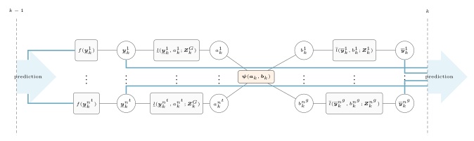
The central box abbreviates $\boldsymbol\psi(\boldsymbol a_k,\boldsymbol b_k)=\prod_{p=1}^{n^t}\prod_{j=1}^{n^g}\Psi_{p,j}(a_k^p,b_k^j)$. Each legacy state has its predicted prior and local likelihood factor. Each group has a newborn state and local likelihood factor; the newborn density is already included in that factor. The observation-only constant $C$ is omitted from the graph.
The factorizations side by side
| Scenario | Association | Extra variables | Factorized joint (up to constants) |
|---|---|---|---|
| S1 point, known $n$ | target-oriented $a_i$, consistency $\psi(\boldsymbol{a})$ | — | $\psi(\boldsymbol{a}) \prod_i f(\boldsymbol{x}_i)\, g(\boldsymbol{x}_i, a_i; Z)$ |
| S2 point, unknown $n$ | target-oriented $a_i$, consistency $\psi(\boldsymbol{a})$ | existence $r$; one new PO per measurement | $\psi(\boldsymbol{a}) \prod_i f(\ub{y}_i)\,\ub{g}(\ub{y}_i, a_i; Z) \prod_j \bar g(\ob{y}_j, \boldsymbol{a}; \boldsymbol{z}_j)$ |
| S3 extended, known $n$ | measurement-oriented $b_i$ (no $\psi$ needed) | Poisson measurement rate $\mu_m(\boldsymbol{y})$ | $\prod_k g(\boldsymbol{y}_k) \prod_i g_{ki}(\boldsymbol{y}_k, b_i; \boldsymbol{z}_i)$ |
| S4 extended, unknown $n$ | measurement-oriented $b_i$ | existence $r$; auxiliary $\tb{y}, \tb{b}, \boldsymbol{\pi}$ marginalized out | $\prod_k \underline q(\ub y_k)\prod_i\underline g_{ki}\;\cdot\;\prod_k\bar q(\ob y_k)\bar g_k\prod_{i>k}\bar h_{ki}$ |
| GrBP extended, preclustered | target-to-group $a^p$ and group-to-legacy $b^j$ | fixed partition; existence; one newborn candidate per group | $C\,\boldsymbol\psi(\boldsymbol a,\boldsymbol b)\prod_p[f(\underline{\boldsymbol y}^p)\underline l_p]\prod_j\overline l_j$ (approximate joint model) |
Two axes of difficulty, two tools. Unknown object number is handled by augmenting states with existence variables and letting each measurement propose a new object. Extended objects are handled by flipping the association direction (measurement-oriented) and giving each object a Poisson measurement count — at the cost, in S4, of a detour through an over-complete representation that is marginalized back out. GrBP instead fixes a preclustered partition and applies exclusive group-to-target association under an approximate clutter-group model.
Before implementing these graphs
- Choose whether the observed data are an ordered vector or a finite set and keep the corresponding combinatorial constants consistent.
- Verify normalization on tiny cases by summing every association and integrating the state variables numerically.
- Keep the birth intensity and birth-state density inside every new-object factor; test that changing either changes birth evidence.
- For S4, enforce $b_i\leq\underline K+i$ and include the $\bar h_{ki}$ factors for later measurements; otherwise a new extended object can generate only its anchor measurement.
- For GrBP, keep one $1/\mu_g$ per target-generated group and retain the detected-newborn zero-truncation factor. Check sensitivity to clustering splits and merges separately from association.
- Compare SPA marginals with exhaustive inference on small scans before using loopy message passing at scale.
References
- F. Meyer, T. Kropfreiter, J. L. Williams, R. Lau, F. Hlawatsch, P. Braca, and M. Z. Win, “Message passing algorithms for scalable multitarget tracking,” Proceedings of the IEEE, vol. 106, no. 2, 2018. (Scenarios 1–2.)
- K. Granström, M. Baum, and S. Reuter, “Extended object tracking: Introduction, overview and applications,” Journal of Advances in Information Fusion, vol. 12, no. 2, 2017. (Scenario 3 measurement model.)
- F. Meyer and J. L. Williams, “Scalable detection and tracking of geometric extended objects,” IEEE Transactions on Signal Processing, vol. 69, 2021. (Scenario 4 construction, supplementary derivation, and factor graph.)